Assessing Highway Tolling and Pricing Options and Impacts: Volume 2: Travel Demand Forecasting Tools (2012)

Below is the uncorrected machine-read text of this chapter, intended to provide our own search engines and external engines with highly rich, chapter-representative searchable text of each book. Because it is UNCORRECTED material, please consider the following text as a useful but insufficient proxy for the authoritative book pages.

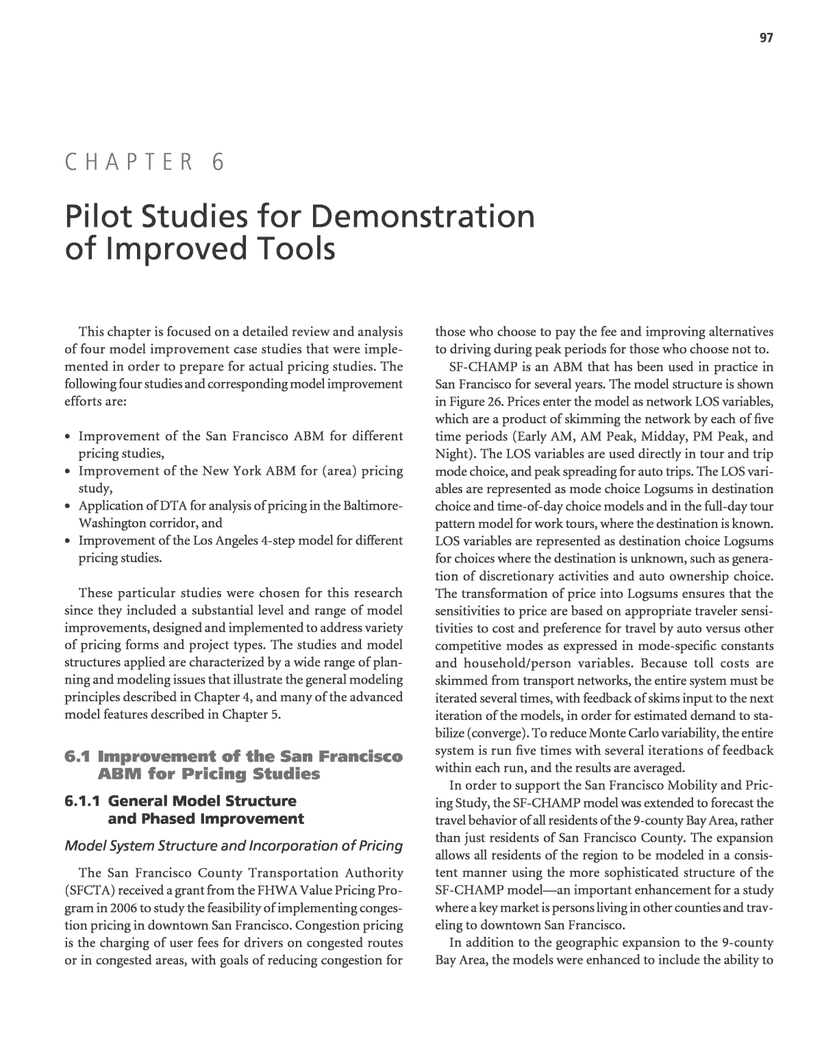
97 This chapter is focused on a detailed review and analysis of four model improvement case studies that were imple- mented in order to prepare for actual pricing studies. The following four studies and corresponding model improvement efforts are: • Improvement of the San Francisco ABM for different pricing studies, • Improvement of the New York ABM for (area) pricing study, • Application of DTA for analysis of pricing in the Baltimore- Washington corridor, and • Improvement of the Los Angeles 4-step model for different pricing studies. These particular studies were chosen for this research since they included a substantial level and range of model improvements, designed and implemented to address variety of pricing forms and project types. The studies and model structures applied are characterized by a wide range of plan- ning and modeling issues that illustrate the general modeling principles described in Chapter 4, and many of the advanced model features described in Chapter 5. 6.1 Improvement of the San Francisco ABM for Pricing Studies 6.1.1 General Model Structure and Phased Improvement Model System Structure and Incorporation of Pricing The San Francisco County Transportation Authority (SFCTA) received a grant from the FHWA Value Pricing Pro- gram in 2006 to study the feasibility of implementing conges- tion pricing in downtown San Francisco. Congestion pricing is the charging of user fees for drivers on congested routes or in congested areas, with goals of reducing congestion for those who choose to pay the fee and improving alternatives to driving during peak periods for those who choose not to. SF-CHAMP is an ABM that has been used in practice in San Francisco for several years. The model structure is shown in Figure 26. Prices enter the model as network LOS variables, which are a product of skimming the network by each of five time periods (Early AM, AM Peak, Midday, PM Peak, and Night). The LOS variables are used directly in tour and trip mode choice, and peak spreading for auto trips. The LOS vari- ables are represented as mode choice Logsums in destination choice and time-of-day choice models and in the full-day tour pattern model for work tours, where the destination is known. LOS variables are represented as destination choice Logsums for choices where the destination is unknown, such as genera- tion of discretionary activities and auto ownership choice. The transformation of price into Logsums ensures that the sensitivities to price are based on appropriate traveler sensi- tivities to cost and preference for travel by auto versus other competitive modes as expressed in mode-specific constants and household/person variables. Because toll costs are skimmed from transport networks, the entire system must be iterated several times, with feedback of skims input to the next iteration of the models, in order for estimated demand to sta- bilize (converge). To reduce Monte Carlo variability, the entire system is run five times with several iterations of feedback within each run, and the results are averaged. In order to support the San Francisco Mobility and Pric- ing Study, the SF-CHAMP model was extended to forecast the travel behavior of all residents of the 9-county Bay Area, rather than just residents of San Francisco County. The expansion allows all residents of the region to be modeled in a consis- tent manner using the more sophisticated structure of the SF-CHAMP model—an important enhancement for a study where a key market is persons living in other counties and trav- eling to downtown San Francisco. In addition to the geographic expansion to the 9-county Bay Area, the models were enhanced to include the ability to C h a p t e r 6 Pilot Studies for Demonstration of Improved Tools

98 Population Synthesizer Vehicle Availability Model Full-Day Tour Pattern Model Discretionary Tour Destination Choice Models Time-of-Day Choice Models Tour Mode Choice Models Intermediate Stop Models Trip Mode Choice Models Workplace Location Choice Model Destination Choice Logsums Zonal Data Network Level-of- Service (including toll costs) Mode Choice Logsums Auto Trip Time-of- Day Choice Model (Peak Spreading) Transit Assignment By Time Period (5) Highway Assignment By Time Period (5 + 30 min. peak intervals) Visitor Trip and Destination Choice Model Iteration + 1 Figure 26. RPM-9 model structure.

99 evaluate cordon pricing and area pricing scenarios at all levels of the decision-making structure. Specifically, this includes the addition of a choice of whether or not to pay a toll to enter the pricing area, the use of a VOT distribution rather than average VOT, and supporting enhancements. After calibrat- ing, these models were used for Phase 2 of the Mobility and Pricing Study. A final set of Phase 3 models was then created to better capture time-of-day shifts expected due to pricing. The Phase 3 models incorporate the information gained from a stated preference survey of persons making auto trips to downtown San Francisco. After implementing these improvements, the model was calibrated to match observed data at a regional level, with a particular focus on San Francisco trips. The resulting models are termed the 9-County Regional Pricing Model (RPM-9). Generalized Cost Assignment in CHAMP 3 For initial study analysis, the one-county CHAMP 3 model was modified to use generalized cost highway path-building, rather than time-only path-building. The generalized cost function is: GenCost Time Occupancy= +0 04 12.  Distance Toll+( ) (Equation 22) In this equation, the 0.04 factor converts from cost in cents to minutes, using an equivalent of $15/hour. The auto operating cost is 12 cents per mile, and toll costs are specified in cents. All costs throughout the model are in 1990 dollars or cents. The division of cost by auto occupancy is new in RPM-9 and allows for the sharing of costs among passen- gers. The auto operating cost is not divided by occupancy because doing so would force the model to predict higher shared ride shares for longer trips, a result that is not seen in the observed data. Expansion to 9-County Area The development of RPM-9 began by modifying the existing CHAMP 3 models to cover the entire 9-county Bay Area. In many cases, such as the application of mode choice models, the same models are applied and calibrated for the 9-county area, only with the removal of a restriction that they apply to only San Francisco residents. In some ways, this makes the entire model system simpler because there is no longer a need to combine the regional results from the MTC model with the SF-CHAMP results. However, to achieve this regional scope, there were a number of changes that needed to be made. Most of these changes involved resolving incon- sistencies between the detailed data that are available only within San Francisco, and the more general data available for the entire 9-county area. 6.1.2 Model Structure Improvement for Choice of Tolls In addition to the expansion to the 9-County area, the behavioral structure of the Phase 2 model was extended to include a choice of tolls. The model updates made as part of that extension are discussed in this section. Networks The highway networks are coded in equivalent manner as the networks for the Phase 1 CHAMP 3.1 models, with one addi- tional field indicating if the toll should be treated as a “value toll” and included as a separate alternative in the choice models. Specifically, the network fields related to tolling are: • TOLLEA_DA – Cost of tolls to single-occupant vehicles in the Early AM; • TOLLEA_SR2 – Cost of tolls to shared-ride 2 vehicles in the Early AM; • TOLLEA_SR3 – Cost of tolls to shared-ride 3+ vehicles in the Early AM; • TOLLAM_DA – Cost of tolls to single-occupant vehicles in the AM Peak; • TOLLAM_SR2 – Cost of tolls to shared-ride 2 vehicles in the AM Peak; • TOLLAM_SR3 – Cost of tolls to shared-ride 3+ vehicles in the AM Peak; • TOLLMD_DA – Cost of tolls to single-occupant vehicles in the Mid-Day; • TOLLMD_SR2 – Cost of tolls to shared-ride 2 vehicles in the Mid-Day; • TOLLMD_SR3 – Cost of tolls to shared-ride 3+ vehicles in the Mid-Day; • TOLLPM_DA – Cost of tolls to single-occupant vehicles in the PM Peak; • TOLLPM_SR2 – Cost of tolls to shared-ride 2 vehicles in the PM Peak; • TOLLPM_SR3 – Cost of tolls to shared-ride 3+ vehicles in the PM Peak; • TOLLEV_DA – Cost of tolls to single-occupant vehicles in the Evening; • TOLLEV_SR2 – Cost of tolls to shared-ride 2 vehicles in the Evening; • TOLLEV_SR3 – Cost of tolls to shared-ride 3+ vehicles in the Evening; • VALUETOLL_FLAG – Binary flag indicating whether or not trips traversing this link should be included in the toll alternative in the choice models.

100 All costs are coded in 1990 cents. The value toll flag is important because it distinguishes between the congestion pricing tolls and the background tolls on the Bay Area bridges. Just because someone is willing to pay a toll to cross the Golden Gate Bridge does not necessarily mean that they are also willing to pay a toll to enter the downtown area. A trip is only included in the toll alternative if it traverses a link where both the value toll flag and the toll for that time period and auto occupancy are greater than zero. If the flag is set to zero, then the toll is still paid, but it is included in the utility equa- tion of the no-toll alternative. Highway shortest paths are built based on the generalized cost (Equation 22). Two separate sets of highway skims are built. The toll skims are allowed to use any link in the net- work, subject to the normal HOV restrictions. The no-toll skims are prevented from using links where the toll and the value toll flag are both greater than zero. The no toll skims include three tables: time, distance, and cost of bridge tolls. The toll skims include four tables: time, distance, cost of bridge tolls, and cost of value tolls. The value tolls need to be skimmed separately such that the availability of toll alterna- tives can be determined, and such that incremental value toll costs can be set to zero for area pricing scenarios. Car Availability, Tour Generation, and Time-of-Day No changes were necessary to the vehicle availability, tour generation, or time of day models in order to accommo- date the revised behavioral structure. Changes were made to achieve better calibration results, however, that are discussed in that section. Tour Destination Choice The tour destination choice and workplace location choice models are integrated with the tour mode choice models, and use the mode choice Logsum as the primary measure of impedance. Therefore, no further changes were required for them to be sensitive to congestion pricing scenarios. Tour Mode Choice The tour mode choice models were re-structured to allow for a more realistic behavioral response to the types of scenar- ios that will be evaluated in the Mobility and Pricing Study. Figure 27 shows the tour mode choice nested structure used by CHAMP 3. This structure is limiting in two ways: First, there is no explicit choice of whether or not to pay the toll, and second it does not necessarily capture differences in cost or toll across auto occupancy. The auto driver alternative in CHAMP 3 is exposed to the drive-alone skims, and the auto passenger alternative is currently exposed to the shared ride 2 skims. In reality, some drivers would be exposed to shared ride skims, and some passengers would be exposed to shared ride 3+ skims. When the scope of the model was limited to San Francisco County without tolling, this was not an issue, but in a region that includes high-occupancy vehicle lanes and toll discounts for carpools, there are some cases where it is limiting. To overcome these issues, RPM-9 uses the nested structure in Figure 28. This structure includes a choice of Drive Alone, Shared Ride 2, or Shared Ride 3+ for greater consistency with the skims. It also includes a choice of toll or no-toll as a sub- nest on each auto alternative. The nesting coefficients for the non-motorized, auto, and transit nests remain at 0.72, and the nesting coefficients on the toll nests are set to 0.50. The resulting product of the nesting coefficients at the lowest level is 0.36, a value consistent with what is typically observed in toll modeling. The utility equations for the toll and no-toll alternatives are the same as the driver and passenger utility equations in the existing model, except that they also include the costs of tolls. The coefficients on toll cost are set to the same as the coefficients other out-of-pocket costs. The nature of the highway skims is such that the toll skims will include a valid path for all OD pairs, but the no-toll skims might not. That is, if it is impossible to reach a TAZ without paying a value toll, then the no-toll pathfinder will not find a path, and the no-toll alternative will not be available. While the toll skims will always have a valid path, the toll alternative Root Auto Driver Passenger Non- Motorized BikeWalk Transit Drive to Transit Walk to Transit Figure 27. CHAMP 3 tour mode choice nested structure.

101 should only be available when toll is a distinct alternative. To meet these criteria, the following rules are defined: • DA No-Toll is available as long as a valid DA path can be found; • SR2 No-Toll is available as long as a valid SR2 path can be found; • SR3+ No-Toll is available as long as a valid SR3+ path can be found; • DA Toll is available if the DA value toll is greater than zero; • SR2 Toll is available if the SR2 value toll is greater than zero; and • SR3+ Toll is available if the SR3+ value toll is greater than zero. These rules are in addition to the existing availability rules: DA not available if it is a 0-vehicle household or age is less than 16. For the congestion pricing scenario, it is expected that for most OD pairs, either the toll or the no-toll alter- native will be available, but not both. The exception to this rule is trips that pass through the congestion pricing area but have the option of avoiding the toll and still reaching their destination. Even though the side-by-side choice of toll ver- sus no-toll is not common, it is still important that the appro- priate alternative be selected in the tour mode choice because that choice will serve as the basis for subsequent models. Toll costs and parking costs are divided by auto occupancy to reflect the sharing of costs among all occupants. Auto oper- ating costs are not shared among occupants, because doing so would result in a model that predicts higher carpooling rates for longer trips, a result not typically observed in reality. The format of the skims also requires that the walk and bike travel times be a function of the distance in the toll skims, rather than the non-toll skims. This will ensure that travelers are not restricted from choosing the non-motorized modes because a toll is imposed. Intermediate Stop Location Choice The intermediate stop choice models previously used the extra time to a stop as the measure of impedance. This extra time is calculated as origin to stop time plus stop to destina- tion time minus origin to destination time. In the CHAMP 3 models, the extra time is specific to the chosen tour mode. During the calibration of CHAMP 3, an extra distance term was introduced such that the models could be calibrated to the average observed trip distance without becoming too sensitive to changes in travel time. For the RPM-9 models, the intermediate stop location choice model was further enhanced to consider the extra toll cost, both of bridge tolls and value tolls. The intermedi- ate stop models use only the toll skims, such that any zone can be reached. With this approach, if the tour mode is toll, then an intermediate stop that would normally require a toll of the same cost can be reached for no additional cost. In the event that the intermediate stop alternative requires paying a value toll both on the origin to stop and on the stop to destination legs of the tour, then an addition cost is incurred. If the tour mode is no-toll, then an intermedi- ate stop that involves paying a toll could still be reached, the cost of paying the toll would be included in the utility. This latter case dictates that individual trip modes can be toll trips, even though the main tour mode was originally chosen as no-toll. Trip Mode Choice With the restructuring of the tour mode choice model, the trip mode choice model receives one of six possible tour modes for auto trips: DA No-Toll, DA Toll, SR2 No-Toll, SR2 Toll, SR3+ No-Toll, or SR3+ Toll. The trip mode choice model assigns each trip in the tour a trip mode in one of the same six categories. It is not required that all trips on a tour have the same trip mode, or match the tour mode. The nested Root Non- Motorized BikeWalk Transit Drive to Transit Walk to Transit Auto Drive Alone Shared Ride 3+ Shared Ride 2 DA No-Toll DA Toll SR3+ No-Toll SR3+ Toll SR2 No-Toll SR2 Toll Figure 28. RPM-9 tour mode choice nested structure.

102 structure for the revised trip mode choice model is identical to the nested structure of the tour mode choice model shown in Figure 28. The upper level nesting coefficients are 0.7 and the toll nesting coefficients are 0.5. Table 17 shows the availability constraints used to con- vert from tour to trip modes. The auto occupancy at the tour level represents the maximum auto occupancy, so at the trip level SR2 tours can have DA trips, but not vice-versa. These availability constraints are defined such that the choice of toll or no-toll at the tour level is non-binding. This non-binding approach is necessary for two reasons. First, not all trips on a toll tour are expected to cross the toll cordon. For example, consider a commuter driving from Palo Alto to downtown San Francisco for work and paying the toll to enter the pricing area. The tour is clearly a toll tour, and the inbound commute is clearly a toll trip. If the toll is only paid on the inbound direction, then the return trip is a no-toll trip. If the commuter stops on the way home in Menlo Park for a softball game, the trip from Menlo Park to Palo Alto is a no-toll trip. Second, it is possible for individual trips on no-toll tours to cross the toll cordon. Consider a commuter driving from the Sunset district to the Presidio for work. This commute does not enter the tolling area and is a no-toll tour. However, after work the traveler drives to the financial district to meet friends for happy hour. This stop is in the pricing area and subject to tolling, so that trip is a toll trip. The trip mode choice model alternatives are also subject to the skim-based availability rules equivalent to the tour mode choice rules. Specifically, these are: • DA No-Toll is available as long as a valid DA path can be found; • SR2 No-Toll is available as long as a valid SR2 path can be found; • SR3+ No-Toll is available as long as a valid SR3+ path can be found; • DA Toll is available if the DA value toll is greater than zero; • SR2 Toll is available if the SR2 value toll is greater than zero; and • SR3+ Toll is available if the SR3+ value toll is greater than zero. As in tour mode choice, these availability rules ensure that in most cases, either the toll or no-toll alternative will be avail- able, but not both. Both might be available in cases where the trip neither starts nor ends in the pricing area, but has the option to go through it. In these few cases, forcing the tour mode to be toll to avoid penalizing travelers twice for paying the same toll might be considered. The toll cost coefficients used in the trip mode choice model are the same as the out-of-pocket cost coefficients. Highway and Transit Assignments For each time period, the highway assignment models read the following eight person trip tables: • DA; • SR2; • SR3+; • Trucks and commercial vehicles; • DA Toll; • SR2 Toll; • SR3+ Toll; and • Trucks and commercial vehicles with toll. After converting the trip tables to vehicle trips, these trip tables are assigned using a multi-class highway assignment. The impedance is the same generalized cost function used for Trip Mode Tour Mode DA No-Toll SR2 No-Toll SR3+ No-Toll DA Toll SR2 Toll SR3+ Toll Walk Bike Walk- Transit Drive- Transit DA No-Toll X X SR2 No-Toll X X X X X X SR3+No-Toll X X X X X X X X DA Toll X X SR2 Toll X X X X X X SR3+ Toll X X X X X X X X Walk X X X X X X X X X X Bike X Walk-Local X X Walk-Muni X X Walk- Premium X X Walk-Bart X X Drive- Premium X Drive-BART X Table 17. Trip modes allowed for each tour mode.

103 skimming, which includes both the cost of bridge tolls and the cost of value tolls. Any HOV restrictions are maintained as is done in the current model. Beyond these HOV restrictions, the toll trip tables are able to traverse any links. The no-toll trip tables will be restricted from traversing links where the value toll flag is greater than zero, and the toll for that occupancy and period is greater than zero. These results are consistent with the paths resulting from skimming. Additional classes of users are introduced for the model’s area pricing mode, as discussed in that section. The introduction of toll nests did not warrant any changes to the transit assignment models. Non-Resident Trips Non-resident trips, including commercial vehicles, exter- nal trips, and visitor trips are not subject to the same behav- ioral framework as normal personal travel. Instead, for each of these components, a binary logit choice model was devel- oped to split the trip tables into toll and no-toll trips. Visitors and external trips use a $15/hour VOT. Commercial vehicles use a $30/hour VOT. Distributed VOT The Phase 2 models were enhanced to include VOT dis- tributions, rather than using fixed average VOT for each income class. In a mode choice model, value-of-time is not an explicit model coefficient, but implied from the ratio of the time coefficient and the cost coefficient. Therefore, there are three possible ways to incorporate a distributed VOT in a mode choice model—using a distributed time coefficient, using a distributed cost coefficient, or using distributed values of both. The utility of money should vary with income, as well as with personal circumstances. It makes sense that a single person earning $60,000 per year would have a different utility for money than someone trying to raise a family of four on the same income. It also makes sense for those two individuals to have very different utilities of time, where one traveler may need to make it to his child’s soccer game, and another may have no specific time restrictions. From a practical standpoint, however, it is not clear what greater effects varying the time coefficient might have, particularly on the user benefit calculations required for New Starts analysis. Since it is safer to vary only the cost coefficient, that approach is taken for RPM-9. Structurally, a work VOT and a non-work VOT are selected for each individual when the work location choice model is run. These VOT are written with the person record in the output file. All remaining models read these VOT and use them in combination with the in-vehicle time co efficient, to calculate the cost coefficient for the model being run. In this way, each individual has a single VOT for work and a single VOT for non-work that are consistent across all models. The method for determining VOT (in 1990 dollars) for each person is: • Divide the household income by the number of full-time household workers plus half the number of part-time household workers. If there is less than one worker in the household, do not divide. The result is the household income per worker. • Divide the household income per worker by 2,080 hours to get the average wage rate per worker for that household. • Construct a log-normal VOT distribution where the mean is half the wage rate for that household, and the sigma is 0.25. Draw from this distribution to obtain the work VOT. • Calculate the non-work VOT as 2/3 the work VOT. • Impose a minimum of $1/hour and a maximum of $50/hour. • For persons less than 18 years old, impose a maximum of $5/hour. • An option is provided in RPM-9 to use the standard, average VOT for each income group. Table 18 shows a comparison of these averages, and the average of the distributed values. The model was calibrated using the distributed VOT, so it is not clear what effect the standard values would have on the calibration results. • VOT distributions for different population and travel segments are shown in Figure 30 through Figure 35. Purpose Income Range Non-Distributed VOT (1989 $/hr) Distributed VOT (1989 $/hr) Work $0-30k $3.61 $3.66 $30-60k $10.82 $8.19 $60k+ $18.03 $16.53 Non-Work $0-30k $2.40 $2.49 $30-60k $7.21 $5.46 $60k+ $12.02 $11.45 Table 18. Comparison of average distributed VOT with non-distributed.

Figure 30. VOT distribution for children. Figure 31. VOT distribution for adults in households with income $0–30k. Figure 32. VOT distribution for adults in households with income $30–60k.

Figure 33. VOT distribution for adults in households with income $60k1. Figure 34. Work VOT distribution for all persons. Figure 35. Non-work VOT distribution for all persons.

Area Pricing Logic Two basic schemes are under consideration for how to oper- ate a pricing system. A cordon approach would require that autos pay a toll any time they traverse a toll link. If a driver entered the pricing area three times in one day, he would be required to pay the toll three times. The second possible scheme is an area pricing approach: once the toll is paid by a vehicle, that vehicle can enter or exit the pricing area an unlimited number of times throughout the day. The mecha- nism to model the area pricing approach is discussed here. A binary flag is included in each of the control files to specify if the area pricing mode should be used. If set to zero, the standard cordon pricing method is used. The model does not allow for a mix of the two approaches; it is one or the other. The basic approach is that tours are sorted first in priority order, then in chronological order. The first time a traveler enters the pricing area, she must pay the full toll. For all sub- sequent travel, there is no toll charged. Changes to the indi- vidual models for area pricing are outlined below. Workplace Location Choice. The workplace location decisions are assumed to be at the top of the hierarchy, so there is no difference from the cordon pricing mode. Tour Generation. The tour generation models are respon- sible for writing the tour records in priority order for each per- son. The work or school tour is always first, followed by all other tours in chronological order. Tour Mode and Destination Choice. The tour mode and destination choice program read the tours in priority order, as written by tour generation. The program stores a variable to keep track of when the person ID changes. Within the tours made by a single person, if any previous tour has chosen a toll mode, a flag is set indicating that the value toll was already paid. If this flag is true, the cost of value tolls in the toll alternative is zero. The rules of operation are: • First (highest priority) tour of the day sees the full toll cost. • If a toll mode is chosen, subsequent tours for that same person have the value toll cost coefficient set to zero. This means that he can go anywhere, for zero additional toll. The coefficient is changed instead of the cost itself, because the toll cost is used to determine if the toll alternative is available. If the toll cost > 0, then the alt is available. • If a person has already paid and the toll alternative is avail- able (with zero toll cost), the non-toll alternative becomes unavailable. The non-toll alternative is unavailable because it is dominated. There is no reason to incur extra time avoiding toll links if there is no need to. Intermediate Stop Location Choice. The intermediate stop location models read the already paid flag created by the tour mode choice models and apply the logic: • If a tour has already paid, the toll cost coefficient is set to zero. Intermediate stops on that tour can stop anywhere for no additional charge. • If tour has not already paid, but the tour mode is toll, then the toll cost coefficient is set to zero, and intermediate stops can occur anywhere for no additional charge. This is distinct from the case above, because the first tour of the day, where the toll must be paid at the tour level. Trip Mode Choice. In trip mode choice, the individual trips on each tour are processed chronologically. The costs are treated normally until the first trip is found that pays the toll. After that point, the value toll costs are zero. Switching is allowed at the trip mode choice level, either from a toll tour mode to a no-toll trip mode, or from a no-toll tour mode to a toll tour mode. The specific logic for area pricing in trip mode choice is: • If the tour is coded as already paid and a toll alternative is available, then any no-toll alternatives are not available, and the value toll cost coefficient is set to zero. • For the first tolled tour of the day (toll tour mode, but already paid is false), the individual trip paying the toll is identified. Each trip is processed in the order that they occur. The ini- tial trip/trips see the full cost until one chooses a toll trip mode. Subsequent trips are given a value toll cost coefficient of zero and treated as having already paid. • Following the choice of modes, any auto trips that have already paid the toll are segregated into separate trip tables such that they can be assigned separately. Non-Resident Trips. The non-resident trip tables are split into toll, non-toll, and already paid, just like the residents. The toll/no-toll choice uses simple logit models, where the VOT is $15/hour for external and visitor trips, and $30/hour for commercial trips. In these aggregate models, it is not possible to explicitly track which trips have paid and have not. Instead, the cost coefficients are divided by the average number of times that the same traveler is expected to enter the pricing area in a day. Lacking any observed data, the model uses the following assumptions: • External travelers enter once per day, • Visitors enter twice per day, and • Commercial vehicles enter twice per day. 106

107 Note that these entries are only the number of inbound trips, assuming that exiting the pricing area is free. Following the choice of the toll or no-toll alternative, the toll trips are split into two trip tables for those who have to pay the toll in assignment, and those who have already paid it. This split is done by dividing by the number of entries per day. Assignment. For consistency with the choice models, four additional user classes are introduced to the highway assign- ment process, bringing the total to 12. The new classes are: • DA Already Paid; • SR2 Already Paid; • SR3+ Already Paid; and • Trucks and Commercial Vehicles Already Paid. These new classes are necessary to avoid further penalizing the vehicles that have already paid the toll. The methods for assigning the trip tables are: • No Toll trips are assigned using the full cost and are not allowed to use any links with a value toll on it. • Toll trips are assigned using the full cost, but are permitted to use any links. • Already paid trips are assigned with zero cost of any value tolls and are permitted to use any links. Feedback Implementation Previous CHAMP models did not include feedback from assignment to the demand models. They were just run once, based on pre-skims created from assigning MTC trip tables. This approach was adequate for many applications, but is lim- iting for the Mobility and Pricing Study. A goal of congestion pricing is to reduce congestion. While travelers with a low VOT are less likely to drive to the pricing area, some travelers with high VOT may be more likely to drive to the pricing area if the travel time savings compensate for the cost. The only way to account for this effect is to feed the travel times from the final assignment back to the skimming process and re-run the models. The details of the RPM-9 feedback approach are described here. Several research presentations on the topic of feedback were reviewed. Each involves some empirical tests for a specific model system and attempts to evaluate what approaches work well for that model. The goal is a method that converges to a stable result in a relatively small number of iterations. The presentations discuss three main topics: • How to measure convergence, • How to combine iterations to achieve convergence, and • How many iterations to run. Slavin, et al. (2007) found that averaging link flows using the method of successive averages seems to work well. Boyce, et al. (2007) advocated averaging trip tables instead of link vol- umes, and found that a constant weight on each new iteration works well. Gibb and Bowman (2007) worked on the Sacra- mento model and used an approach where they started with a small sample in the demand models for early iterations and increased the sample sizes with later iterations. Vovsha, et al. (2008) advocated averaging both trip tables and network vol- umes based on the experience with the New York model. The approaches presented found generally good convergence in the range of 4-10 iterations, with declining returns for increases in the number of iterations. They all emphasized that their results are not necessarily transferable and that they should be tried with a specific model system to see what works best. Given this information, the following approach was imple- mented for RPM-9. The approach may be modified as the model is tested and used if its behavior warrants. 1. Call all of the initialization scripts, and run the first assignment using MTC trip tables (implemented in run- Model.bat). 2. Run an iteration of the demand models and assignments, given a specified iteration number, weight for combining the previous and next iterations, and sample rate (imple- mented in runIteration.bat). Each iteration includes the following steps: – Each iteration runs everything from the highway skims through the highway assignment. – The core models are run with the specified sample rate. They are run six times and averaged, since there is little incremental cost given the distribution across multiple machines. – At the end of the iteration, the link volumes of the result- ing networks are averaged with the link volumes on the input network using the weights specified. – A report is written (to feedback.rpt) showing the differ- ences in the assignment results and the differences in the trip tables. – The averaged networks are renamed to serve as the basis for skimming for the next iteration, and the trip table is copied for comparison after the next iteration. – All other files are over-written during the next iteration. 3. RPM-9 runs a fixed number of iterations. Using a fixed number should make scenarios more comparable if results fluctuate a bit from iteration to iteration. It runs four itera- tions with the parameters shown in Table 19. 4. On the first iteration, there is zero weight given to the previous assignment, because it is based on the MTC trip tables, not the SF-CHAMP trip tables. On the final itera- tion, the networks are still averaged, but the final assigned networks are kept.

108 6.1.3 Model Estimation and Structural Changes After the interim Phase 2 models were completed, the RPM-9 was further enhanced to more realistically capture travelers’ time-of-day responses to pricing, an important consideration for the study team. At the same time, the tour generation models and vehicle availability models were modified to account for the potential suppression of trips due to pricing, and the VOT distributions were estimated from stated preference survey data. SP Survey In July and August 2007, Resource Systems Group administered a survey of travelers driving to downtown San Francisco. The SP survey was designed to help understand traveler’s response to a potential entry fee into the down- town area. A total of 663 respondents completed a series of experiments, where they traded off cost, shifted their trip time, or changed to transit. The full report is available in RSG (2007). Model Sequencing The sequencing of time-of-day choice within the travel models is a classic chicken-and-egg problem. When choosing a time-of-day, one might expect that travelers would consider the travel time between their origin and destination for the mode they have chosen. For example, auto trips might be likely to shift out of the peak due to congestion, but transit trips might be likely to shift into the peak due to the higher frequency of transit service. Accounting for this would require knowledge of both mode and destination. Similarly, when choosing a mode, travelers might consider their origin, destination, and depar- ture time. Finally, when choosing a destination, travelers may be sensitive to mode and departure time. One approach to resolving this issue would be to build a joint mode, destination, time-of-day choice model. Such a model, however, would have a large number of alternatives, and likely be unwieldy and difficult to calibrate. Another good approach, and the one used here, is to assert a priori logical sequencing of choices, and to use Logsums from downstream models in the upstream choices. The project team believes that the most logical sequencing of these three choices within the RPM-9 framework is: 1. Destination choice, 2. Time-of-day choice, and 3. Mode choice To accomplish this sequencing, the time-of-day choice model uses mode choice Logsums for the time-of-day alter- natives being considered. The destination choice model could use time-of-day Logsums as a measure of impedance between zones, but this would break the traditional understanding of how a destination choice model works and enter a level of theoretical abstraction with which the project team was not comfortable. Instead, the destination choice model works by starting from initial simulated times-of-day for each tour and choosing a destination by considering the mode choice Log- sums for that initial time-of-day. The time-of-day model then replaces the initial time-of-day with the actual chosen time-of- day. The only purpose of the initial simulated time-of-day is to provide a basis for destination choice, so the details of how those are determined are not particularly important. In this case, the old time-of-day model from CHAMP 3 is run, which provides a simulated distribution equivalent to the actual dis- tribution. In this way, the chicken-and-egg problem is resolved and the models operate in a consistent manner. The final sequencing of all models is: 1. Choose a workplace location, assuming an AM peak departure, PM peak return, and autos greater than or equal to workers. 2. Choose the vehicle availability, considering the destination choice Logsum at home, at work, and the mode choice Logsum between home and work. 3. Run tour generation, with consideration for the destina- tion choice Logsum at home, at work, and the mode choice Logsum between home and work. 4. Determine the initial simulated time-of-day using the CHAMP 3 time-of-day model. 5. Choose primary destinations for non-work tours, con- sidering the initial simulated time-of-day and the mode choice Logsum. 6. Choose the tour time-of-day for all tours, considering the chosen destination, and mode choice Logsums. Iteration Sample Rate Weight for Previous Link Volumes Weight for Current Link Volumes 1 8 0 1 2 4 0.5 0.5 3 2 0.67 0.33 4 1 0.75 0.25 Table 19. Averaging parameters for each feedback iteration.

109 7. Choose the tour mode, considering the chosen destination and chosen time-of-day. 8. Choose locations for any intermediate stops. 9. Run trip mode choice given previously chosen primary and intermediate destinations, previously chosen times-of-day, and the previously chosen tour mode. 10. Assign highway and transit trips. 11. Run the trip time-of-day model (explained in more detail below) to allocate auto trips to more detailed sub-periods. Tour Time-of-Day Choice For each tour, the tour time-of-day choice model chooses the departure time from home, and the departure time from the primary destination. The time periods used are the five periods consistent with the skims: • Early AM (EA): 3:00-5:59 AM, • AM Peak (AM): 6:00-8:59 AM, • Midday (MD): 9:00 AM-3:29 PM, • PM Peak (PM): 3:30-6:29 PM, and • Evening (EV): 6:30 PM – 2:59 AM. The return time period must be the same as or later than the departure time period. Therefore, the model has 15 alternatives: • EA to EA, • EA to AM, • EA to MD, • EA to PM, • EA to EV, • AM to AM, • AM to MD, • AM to PM, • AM to EV, • MD to MD, • MD to PM, • MD to EV, • PM to PM, • PM to EV, and • EV to EV. This structure is equivalent to the old time-of-day models, except that it is applied for all tours, not just for the primary tour of the day. Tours are scheduled first in priority order, then in temporal order. Therefore, if there is a work or school tour, that is scheduled first, followed by any other tours, then any work-based sub-tours. If there is more than one other tour, they are scheduled in the order they occur in the initial sim- ulated times-of-day. Secondary tours are subject to the time constraints imposed by previously scheduled tours, thus pre- venting any overlap. For example, if a work tour has already been scheduled for the AM to PM, then another tour that is being scheduled can occur in the AM to AM or the PM to PM or the PM-EV, but it cannot occur in the MD to PM or EA to EV because that would conflict with the work tour. Sub-tours must be within the bounds of their parent tour. Trip Time-of-Day Choice The trip time-of-day model determines a detailed departure time for each auto trip. Within the peak periods, the resolution is half-hour periods. Outside of the peaks, more aggregate periods are used. In addition to the highway travel time and cost for each sub-period, the model considers the amount of shift from the desired departure time. This model structure corresponds to the format of the stated preference survey, where respondents were asked about a recent trip they made to downtown San Francisco, and what they would do if prices were imposed for different time periods: shift before the pricing period, shift after the pricing period, or switch to transit. For example, if the desired departure time is 8:00 AM, and the alternative being considered is a 9:00 AM departure, then the shift is 60 minutes. Figure 36 shows the effect of time shifts on the utility function. When the trip time-of-day model was implemented within the RPM-9 model stream, it is run after the trip mode choice model, not jointly with mode choice as in the estimation above. It is run using half-hour periods in the peaks, a one-hour buffer at the edge of the peaks, and more aggregate periods in the off peaks. The temporal alternatives are: • EA300: 3:00–4:59 AM, • EA500: 5:00–5:59 AM, • AM600: 6:00–6:29 AM, • AM630: 6:30–6:59 AM, • AM700: 7:00–7:29 AM, • AM730: 7:30–7:59 AM, • AM800: 8:00–8:29 AM, • AM830: 8:30–8:59 AM, • MD900: 9:00–9:59 AM, • MD1000: 10:00–10:59 AM, • MD1100: 11:00 AM–1:29 PM, • MD130: 1:30–2:29 PM, • MD230: 2:30–3:29 PM, • PM330: 3:30–3:59 PM, • PM400: 4:00–4:29 PM, • PM430: 4:30–4:59 PM, • PM500: 5:00–5:29 PM, • PM530: 5:30–5:59 PM, • PM600: 6:00–6:29 PM, • EV630: 6:30–7:29 PM, and • EV730: 7:30 PM–2:59 AM.

110 The model considers the tour time-of-day, and requires that the chosen trip time-of-day be within 1 hour of the tour time. For example, a trip whose tour time is AM peak can choose EA500, any alternative within the AM peak, or MD900. To deal with the shift variables appropriately, a desired departure time is chosen for each trip from the observed dis- tribution of departure times within each main period. Once this desired time is chosen, then a shift can be calculated for any alternative. Travel times for each alternative are derived by: 1. Starting from the loaded highway networks output from assigning trips for the five main periods. 2. Factoring the main period volumes into sub-period vol- umes using constant factors on all links, derived from traffic counts. 3. Factoring the main period tolls into sub-period tolls using factors specified by the user. This allows the user to model a higher toll for the peak-of-the-peak. 4. Skim the shortest paths for each sub-period based on these factored networks. The detailed temporal distribution for factoring is derived from traffic counts, as shown in Figure 37. Hourly traffic counts were available on state highways from Caltrans, and 15 minute counts were available for a cordon around the pric- 0.50 - 1.00 1.50 2.00 2.50 3.00 3.50 4.00 4.50 5.00 -120 -100 -80 -60 -40 -20 0 20 40 60 80 100 120 D is ut ili ty Shift from desired departure. min Commute AM Other AM Other PM Figure 36. Effect of time shift on utility. Figure 37. Diurnal traffic count distribution.

111 Variable Coef. Std. Err. z Parameter Prob > z 95% Interval Conf. (lower & upper bounds) Mean cost0_30 -0.2884 0.0456 -6.33 0.000 -0.3777 -0.1990 cost30_60 -0.1968 0.0193 -10.20 0.000 -0.2346 -0.1590 cost60_100 -0.1661 0.0151 -11.02 0.000 -0.1956 -0.1365 cost100p -0.1349 0.0119 -11.33 0.000 -0.1582 -0.1115 shift_earl~r -0.0126 0.0012 -10.85 0.000 -0.0149 -0.0103 shift_later -0.0206 0.0022 -9.53 0.000 -0.0248 -0.0164 delay_1_5 -0.0127 0.0062 -2.07 0.039 -0.0248 -0.0007 delay_1_10 -0.0050 0.0063 -0.79 0.430 -0.0173 0.0073 transitWalkTime -0.0307 0.0044 -6.95 0.000 -0.0393 -0.0220 transitDriveTime -0.0307 0.0111 -2.75 0.006 -0.0525 -0.0088 transitFreq -0.0166 0.0071 -2.34 0.019 -0.0304 -0.0027 transitXfers -0.2434 0.0889 -2.74 0.006 -0.4176 -0.0693 transitDrive -0.4426 0.1639 -2.70 0.007 -0.7637 -0.1214 bart -0.0180 0.1659 -0.11 0.914 -0.3432 0.3072 caltrain 0.2834 0.1889 1.50 0.133 -0.0868 0.6537 muniMetro -0.0851 0.1653 -0.52 0.607 -0.4091 0.2388 prepeak 0.2987 0.0891 3.35 0.001 0.1241 0.4733 postpeak -0.5271 0.1013 -5.20 0.000 -0.7257 -0.3286 transitAlt -0.2223 0.2014 -1.10 0.270 -0.6170 0.1725 travel_time -3.9231 0.2338 -16.78 0.000 -4.3813 -3.4649 Standard Deviation travel_time 0.8709 0.3215 2.71 0.007 0.2408 1.5010 Ratios to Mean In-Vehicle Time Walk Time 1.06 Drive Time 1.06 Transfers 8.42 Wait Time 3.49 Constants Prepeak -10.34 PostPeak 18.24 Transit 7.69 Bart 0.62 CalTrain -9.81 Muni Metro 0.34 Time Coefficient Statistics Median -0.01978 exp(coef) Mean -0.0289 exp(coef + sd^2/2) Standard Dev -0.03079 mean * sqrt(exp(sd^2) -1) VOT by Income Group Median Mean 0-30k $4.12 $6.01 30-60k $6.03 $8.81 60-100k $7.15 $10.44 100k+ $8.80 $12.86 Table 20. Trip time-of-day mixed logit estimation results. ing area. The downtown counts were shifted somewhat from the regional counts, so the detailed downtown area counts were adjusted to better match the regional distribution. VOT Estimation The SP data were also used to estimate VOT distributions for use throughout the model stream. This was done by estimating a joint mode and departure time choice model, except with mixed logit, rather than nested logit. Mixed logit is important in this case because it allows the user to estimate a distribution on a coefficient, rather than just the mean value. In this case, a distribution was estimated on the travel time variable, assert- ing a lognormal form. The cost coefficients are estimated as standard, nondistributed coefficients segmented by income. The resulting model is shown in Table 20. The most important result of this estimation is the mean and median VOT shown at the bottom of the table. When the estimated VOT distributions are plotted as log- normal functions the curves are the shapes shown in Figure 38. These distributions are used in RPM-9 and replace those used in the Phase 2 models. 6.1.4 Model Calibration After implementing the structural changes, RPM-9 was calibrated to match observed data for the 9-county area.

112 Figure 38. VOT distributions estimated from mixed logit. Period Percent in Peak Hour EA 46.3% AM 34.8% MD 15.4% PM 33.7% EV 17.3% Table 21. Revised peak-hour percentages for assignment. The following section discusses the calibration process, final model coefficients, and comparisons to observed data. The calibration targets were derived from the 2000 Bay Area Travel Survey (BATS 2000). They are generally in the same format as the targets used to calibrate CHAMP 3, but are not restricted to only San Francisco residents. An extended set of traffic counts was used to validate the highway assignment results. The previous CHAMP 3 count database included 1,091 counts, all within San Fran- cisco. An extended database was created with an additional 617 counts in the remaining eight counties. These counts are from the Caltrans hourly count database, for the years 1998 through 2000. SFCTA staff coded each count to the network links. Additional observed transit data were provided by MTC, and are the same as those used to calibrate the 2000 base year for the MTC model. These data include boarding counts for each transit operator in the region. Previous (CHAMP 3) calibration efforts focused on miti- gating the initial under-prediction of highway volumes at a system-wide level. Building upon that successful calibration, the RPM-9 calibration moved to the next level, and focused on calibrating to bridge volumes and screenline volumes by time-of-day. In mitigating this issue, a number of modifica- tions were made to the model system: • Updated the factors used to convert from the total period volume to the hourly volume within the period based on recent traffic counts. Table 21 shows the revised peak hour percentages used for assignment. • To balance the above change, and maintain appropriate congested travel speeds, introduced an adjustment factor of 1.2 applied as a product to the volumes in the volume- delay functions. • Upgraded Embarcadero, Sunset, and Great Highway to super-arterials, reflecting divided medians and lower cross traffic. • Converted Golden Gate Bridge and Bay Bridge from Area Type 3 (urban) to Area Type 1 (CBD), reflecting their narrow lanes and lower speed limits. • Converted the Bay Bridge Toll Plaza to Facility Type 5 (ramp), reflecting a lower capacity at the plaza. • Shifted commercial vehicle and internal-external trips in the markets that cross the Bay Bridge or Golden Gate Bridge out of the peak periods. 6.1.5 Conclusions The SCFTA case study demonstrates how an ABM can provide clear advantages over trip-based models in the anal- ysis of pricing policies. The limitations of trip-based models (lack of policy sensitivity and insufficient market segmenta- tion) can be overcome with more advanced models such as SF-CHAMP. There are, however, a number of issues that remain to be addressed by ABMs in practice. First, this model, like most ABMs, relies on static equilibrium high-

113 way assignment algorithms. It is common knowledge that such techniques fail to adequately address congestion due to their lack of ability to reflect queuing. One of the advan- tages of priced facilities (particularly dynamically priced facilities) is that they offer more reliable travel times than competing congested facilities where the variability of travel time can be quite onerous. We need better tools to reflect reliability and address the value of reliability on travel deci- sions. The impacts of pricing on long-term choices such as vehicle ownership, workplace location, residential location, and ultimately firm location need to be better understood. Most ABMs are based on cross-sectional data and unable to fully capture the long-term behavior associated with the introduction of pricing policies. Hopefully as more poli- cies become implemented, more data will be available to improve this critical aspect of travel demand models. 6.2 Improvement of the New York ABM for Manhattan Area Pricing Study 6.2.1 Objectives of the Study Area Pricing Concept in New York This section reviews the demand modeling that has been done with adaptations of the New York ABM for the planning and analysis of New York City’s PlanNYC and its congestion pricing component in particular. The modeling of a Conges- tion Pricing Zone (CPZ), or a proposed area pricing concept for the Manhattan CBD similar to the London pricing scheme, began with work done for the New York City Partnership in 2005 and evolved in the subsequent modeling in support of the development of the City of New York’s long range transporta- tion investments plan or “PlanNYC 2030” in 2006-2007. In this work, and in the subsequent Pricing Commission review phase mandated by the New York state assembly its approval of the City’s submittal of an Urban Partnership Agreement grant application in mid-2007, the new York ABM was adapted and refined to assess congestion reduction and other transporta- tion impacts associated with various proposed pricing options, as well as for alternative strategies aimed at achieving similar levels of congestion reduction for travel to, from, and within Manhattan. The nature and variety of pricing forms and policies con- sidered in the study represented a real challenge from the modeling standpoint. To accomplish this, a number of modeling enhancements and refinements to the standard New York ABM platform were developed and applied to sup- port the estimation of impacts on different traveler markets and various transportation system performance measures. These modeling improvements allowed for better under- standing of the likely behavioral responses to the changes in road pricing and congestion levels associated with Manhat- tan congestion management programs. The congestion pricing, tolling, and other congestion miti- gation strategies that required evaluation and modeling for New York City’s planning comprised a fairly wide range and challenging set of transportation policies and actions as described in the next section. The modeling and evalua- tion of these pricing alternatives and other policies needed to address a spectrum of related transportation issues, within the complexity of the New York Metropolitan Region, including many that are unique in comparison to the other metropolitan regions. In particular, the following aspects were of primary importance: • Transit service to and from Manhattan is extremely devel- oped from most areas of the region. The current transit share in commuting to and from Manhattan is close to 80%. As such, transit represents a very good alternative to the auto for commuters and other travelers to Manhattan, but since most of the transit lines are already crowded in peak hours, very little transit capacity is available to accommodate additional riders who might be influenced to switch from driving due to congestion pricing. • Existing auto commuters to the CBD represent a special market that needs to be well understood before any policy could be seriously considered. Some of them (although not the majority) may be considered “captive” users for either of two reasons. For most of the existing auto com- muters, surveys have shown that employer and other subsidies are prevalent with respect to parking cost, tolls, and vehicle operating cost, making the use of a car com- pelling. In addition to these drivers, the most substan- tial share of auto commuters to CBD comes from “outer boroughs” of New York City, where transit service from these areas is the most limited, without walk to subway or commuter rail options. • Residence of commuters and other travelers to Manhattan is important since some other pricing policies are differ- entiated by the place of residence. From this point of view, three major segments could be distinguished: 1) residents of Manhattan who contribute to intra-Manhattan reverse commuting out of Manhattan, 2) residents of other four New York City boroughs who contribute to relatively short commute trips to Manhattan, and 3) residents of outer sub- urbs from four states (New York, New Jersey, Connecticut, and Pennsylvania) who contribute to longer commute trips to Manhattan. Congestion Pricing Zone (CPZ) Geographically, the Manhattan CPZ was defined as part of Manhattan South of 60th Street; see Figure 39. This definition

114 was more conservative compared to the previously imple- mented (preliminary) study where the border was at the 86th street. The CPZ has several portals (bridges and tunnels) con- necting it to the rest of the metropolitan region. They can be grouped in the following way: • Tolled bridges and tunnels of the Metropolitan Transit Authority (MTA), • Tolled bridges and tunnels of the Port Authority of New York and New Jersey (PANYNJ), and • Free bridges of the New York City (NYC). In addition to the set, there are the Harlem River bridges that are not directly connected to CPZ, but are still relevant choices for some travelers to and from Manhattan. 6.2.2 Modeled Options for Area Congestion Pricing Main Area Pricing Options and Other Strategies Modeled The study considered a wide spectrum of pricing forms and policies where each scenario was defined as a combina- tion of the following main characteristics: • Type of charge. Alternatives included daily fee paid once a day regardless of the number of trips to CPZ (i.e., daily permit) and (recurrent) toll paid for each trip. • Rate charged. Alternatives were formulated in terms of the amount charged, flat versus variable tolls by time of day, pricing schedule (12 hours, 24 hours, etc.), and toll off- Figure 39. Manhattan CPZ and existing bridges and tunnels.

115 set (full or partial credit) for travelers who already paid a creation toll on one of the MTA or PANYNJ tolled cross- ings. Sub-alternatives included surcharges for non-EZ- pass vehicles (based on license plate reads) and surcharges for taxi trips. • Northern boundary of CPZ. Alternatives included 86th St. and 60th St. • Policy for intra-zone trips. Alternatives included free, dis- counted, and full-fee options for staying in CPZ. • Policy for through trips. Alternatives included providing a free peripheral route around CPZ on FDR Drive and Rt. 9A or charging on it. • Trip direction charged at cordon crossings. Alternatives included 2-way (inbound and outbound) tolls and 1-way (inbound only) tolls. • Differentiation by vehicle type. Alternatives included dif- ferent specific toll schemes for trucks and taxis compared to the base fee for auto. In the course of the study, several additional pricing and congestion-mitigation strategies were formulated and required modeling: • Higher tolls on existing tolled Manhattan crossings (MTA and PANYNJ). • Introduce tolls on the currently free Manhattan bridges. Alternatives included a subset of four East River free bridges or all Manhattan bridges (including Harlem River and Henry Hudson). • License Plate Rationing. Alternatives included different ways to impose prohibitions on entry to CPZ by vehicle license plate number. They included either 10% or 20% of vehicles for each day. • Parking Policies. Alternatives included reduction in free parking permits for City employees (targeted zones in CPZ) and elimination of Manhattan resident parking tax rebates. The main characteristics of the CPZ scheme are summarized in Table 22. The initial plan has undergone a substantial revi- sion with regard to such characteristics as the North boundary, direction of charge, imposing of intrazonal charge, providing a free periphery, charging taxis, and license plate rationing. Modeling Challenges Associated with Area Pricing The ABM developed for the New York Metropolitan Transportation Counsel (NYMTC) and first deployed for planning in 2001 was used as the modeling platform for the area pricing study. Some of the pricing forms studied could be addressed adequately with little or no modification of the model, due to the structural advantages of the NYMTC ABM and its ability to model individual household, person, and tour/ trip records in the microsimulation fashion. For those pricing features that required new methods to be introduced, the ABM structure allowed for the addition of incremental improve- ments in a natural and consistent way. For example, for the license plate rationing options, in which the number of vehicles in each household is modeled endogenously and auto avail- ability for each member of the household is explicitly evalu- ated in the mode choice model, it was possible to introduce new controls to test these strategies that mirror the logic of actual travel decision-making, in this case focused on the initial stage of modeling intra-household car allocation and subsequent use by affected households. In this sense, the ABM and the microsimulation implementation of it contributed both to the generation of more reliable estimates of impacts than a conventional aggregate model could, as well as offered the ability for the planner to report and explain these responses logically, and in considerable detail for specific travel markets of concern, e.g. low-income population, residents of specific neighborhoods, and tour types. Another important advantage of the NYMTC ABM is that it considers travel tours as units for mode, destination, and time- of-day choice decisions. This ensures realism and consistency of the modeled choices. It is fundamentally different from the trip-based models that do not recognize internal linkages across the trips in the same tour and can result in conflicting choices of modes and destinations for different trips made by Characteristic Initial plan Final recommendation Daily fee or toll per trip Daily fee Daily fee Duration 12 hours (6 AM – 6 PM) 12 hours (6 AM – 6 PM) Flat or variable & amount Flat $8 Flat $8 North boundary 86th St. 60th St. Direction of charge 2-way In-bound Intrazonal charge Yes No Through trips Free periphery No free periphery Toll offset Yes Yes Taxis Free $1 trip charge License Plate Rationing surcharge None Yes 1$ Table 22. Characteristics of the CPZ.

116 the same person as parts of the same tour. In the context of area pricing, this consistency of the NYMTC ABM was of primary importance since it allowed for capturing impacts of pricing applied for one time-of-day period (for example, the AM peak period) on the other periods of the day (for example, PM when the return commuting mostly occurs). Aside from the ABM issues, special network methods were also developed to address the single fee policy feature of area congestion pricing, i.e., a one-time charge or permit to travel to or within the charged zone for some designated period of time, in contrast to the simple toll transaction-based charges that are easily implemented, for both network skimming and assignment by means of toll link attributes. While a full and logical implementation to address this unique aspect of an area charging fee would be possible in the ABM structure that oper- ates with entire day individual patterns, due to time and budget limitations, a simple scaling of cordon link fee tolls, reflecting daily trip frequencies for different tour types, was applied. A related, but even more difficult issue, was the need to consider and credit tolls paid on existing tolled crossings into Manhattan, such as those operated by PANYNJ and MTA. For example, in some scenarios, the policy to be tested might be an $8 cordon fee, but with the $5 EZ-pass toll paid at the Lincoln Tunnel credited, the effective cost for a driver using the tun- nel to enter the CPZ would be only $3. Using link-based tolls with the standard highway network procedures found in exist- ing modeling platforms requires various configurations of dummy links for these toll increments associated with crossing the cordon and reflecting the upstream tolls. Corresponding procedures were developed, generally resulting in a realistic representation of the policy with respect to costs that travelers would consider in their destination, mode, and route choice. A more robust implementation may be the application of node to node based toll algorithms, not yet tested in this application. As part of this work, aspects of the available data and ele- ments of the modeling technology that could be further refined to increase the precision and level of confidence of the forecasts have been identified. These included more specific methods of representing and modeling a complex system of cordon fees and tolled crossing credits, as well as time-of-day choice model sensitive to tolls and congestion levels, and responsive- ness to specific parking policies and pricing. These additional enhancements could be implemented within the New York ABM and could serve to further increase levels of confidence in the planning forecasts, as well as to possibly support an invest- ment grade level of T&R forecasting and analysis. 6.2.3 Structure of the NYMTC ABM General Model System Structure The NYMTC ABM represents an advanced structure that is based on tour-based and activity-based modeling principles applied in a micro-simulation fashion. This model allows for detailed and behaviorally realistic analysis of traveler responses to pricing. The NYMTC ABM structure is presented in Figure 40 [see also NYMTC (2004) for a more detailed technical description]. It has four major modules applied consecutively with possible feedbacks involving all or some of the modules: • Tour generation that includes household synthesis, auto ownership, and tour frequency choice models, • Tour mode and destination choice that includes pre-mode choice between motorized and non-motorized travel, pri- mary destination choice, entire tour mode combination choice, stop-frequency choice, and stop-location choice, • Time-of-day choice and pre-assignment processor that include tour time-of-day allocation for outbound and inbound directions, and aggregation tours and stops micro- simulation results to mode and time-of-day period trip tables, • Traffic and transit network simulations (assignments) that are implemented by mode and vehicle class, by time- of-day periods. The first three modules are implemented as fully-disaggre- gate micro-simulation procedures working with individual records for the synthesized population (households, persons, tours). The last module is currently based on standard aggre- Tour Generation Mode & Destination Choice Time-of-Day Choice Assignments M ic ro -S im ul at io n Household Synthesis Auto Ownership Tour Frequency Pre-Mode Choice Non-Motorized Motorized Destination Destination Mode Stop Frequency Stop Location Stop Density Logsum Mode Choice Logsum Density Logsum Outbound / Inbound Time Trip Mode Choice Trip Tables Construction Highway Transit H ig hw ay L O S Tr an si t L O S Figure 40. Structure of the NYMTC ABM.

117 gate (zone-to-zone) assignment algorithms. The application software supports numerous feedbacks to be implemented until equilibrium is reached. LOS skims after the last stage can be fed back to the mode and destination module, as well as to the tour-generation components through accessibility indices. The tour-generation module of NYMTC ABM model consists of three successive models that include a household population synthesizer, an auto-ownership model, and a tour- frequency choice model. The household synthesis is based on the predetermined socio-economic controls (number of house- holds, population, labor force, and income) for each zone. The auto ownership choice model is applied for each household and is sensitive to the household characteristics and residential zone accessibility by auto and transit respectively. The tour- frequency model is implemented at the person level. There are three person types and six travel purposes that yield 13 tour fre- quency models taking into account that children cannot make tours to work, at work or university tours; and non-working adults cannot make tours to work or at work. Each model is essentially a multinomial logit construct having three choice alternatives (no tours, one tour, two or more tours). The set of the tour-frequency models is ordered and linked in such a way that choices made for some purposes and household members have an impact on the other choices of the same person, as well as for the other household members. The mode and destination module starts with a pre-mode choice step, where each tour is assigned to either motorized or non-motorized mode of travel. Density of non-motorized attractions is essentially a log-sum from the subsequent destination-choice model for non-motorized travel with individual attractions available in a 3-mile radius around the tour origin. If the motorized option is chosen, then the motorized branch of the algorithm is activated. First the mode and primary destination choice for the entire tour is modeled (without intermediate stops). It can be thought of as a nested structure where destination choice comes at the upper level of the hierarchy, while mode choice is placed at the lower level conditional upon the destination choice. The motorized destination choice model has been cali- brated by eight purposes (six original purposes with additional subdivision of work tours by three income categories). In the microsimulation framework, the destination choice model is applied as a doubly constrained construct (either fully con- strained or relaxed constrained). Constraining the destination ends is achieved by removing the chosen (taken) attraction from the zonal size variable after each individual tour simu- lation. For fully-constrained mandatory purposes (work, school, university), an entire attraction unit is removed. For relaxed constrained non-mandatory purposes (maintenance, discretionary, at work), only a part (0.5) of the attraction unit is removed. The mode-choice model has been estimated for six purposes as a nested logit construct with differential nesting depend- ing on the purpose. In most cases, drive-alone and taxi modes proved to be in separate nests, while transit and shared-ride mode were nested in different combinations. In the next stage of the motorized branch of the application, intermediate stops are modeled conditional upon the chosen mode and primary destination for the tour. Stops are modeled by means of two linked choice models: stop frequency and stop-location. The stop-location model includes a zonal stop- density size variable that is similar to the attraction size vari- able. The composite log-sum from the stop-location model is used in the upper level stop-frequency model. The stop-frequency model has been calibrated for six pur- poses as a multinomial logit construct. After having consid- ered observed stop frequencies from the survey (it was found that an absolute majority of tours do not have more than one stop on each leg of the tour ( 90-95%, depending on the tour purpose), a decision was made to limit the number of choice alternatives to the following four: 1 = no stops on either out- bound or inbound direction; 2 = one outbound (from home) stop leg, no inbound (return home) stops; 3 = no outbound stops, one inbound stop, and 4 = one stop on each direction. The stop-location choice model is also a multinomial logit construct. Similar to the destination-choice model, the stop-location model requires a procedure for selecting a limited subset of relevant zones (for both model calibra- tion and application) in order to reduce the computational burden. For the stop-location model, however, both the OD of the tour are known from prior processing, thus effective rules were applied to build a spatial envelope that reflects the observed stop patterns. The current version of the NYMTC ABM has a simple time- of-day model based on a set of predetermined time-of-day distributions segmented by travel purpose, mode, and des- tination area. One of the identified for further enhancement of the NYMTC ABM includes replacement of the time-of-day distribution with a time-of-day choice model sensitive to per- son, household, and LOS variables. Currently, time-of-day allocation is followed by trip-level mode choice (in most cases predetermined by the entire-tour mode) and a pre-assignment processing procedure that aggregates the microsimulation results and constructs mode-specific and period-specific trip tables. Segmentation and Level of Network Details The basic version of NYMTC ABM, which was used as the platform for the model improvements implemented for the pricing analysis, has the following main structural dimensions: • Eleven travel modes (drive alone, shared ride-2, shared ride-3, shared ride-4+, transit (including bus, subway, and ferry) with walk access, transit with drive access, commuter rail (with transit feeder lines) with walk access, commuter rail with drive access, taxi, school bus (for tours to school only), and walk (the only non-motorized mode),

118 • More than 100 population segments including a Carte- sian combination of three household income groups (low, medium, high), four household car-sufficiency groups (without cars, cars fewer than the number of workers, cars equal to workers, cars greater than workers), and three person types (worker, non-working adult, child), • Six travel purposes including work, school, university/ college, household maintenance (shopping, banking, escort- ing children, visiting a doctor), discretionary activity (leisure, entertainment, visiting relatives and friends, eating out), and non-home-based sub-tours originated and ended at work (as a special segment), • Two freight traffic components that are characterized by a distinctive value of time and willingness to pay: heavy trucks with 3+ axles and light trucks (commercial vehicles) with 2 axles. • Four time-of-day periods (AM peak 6:00–10:00, midday 10:00–16:00, PM peak 16:00-20:00, and night 20:00–24:00, 0:00–6:00). • Six vehicle classes applied in the multi-class highway assignment including SOV, HOV-2, HOV-3+, light trucks and commercial vehicles, heavy trucks, and external auto trips to, from, and through the region are allocated by vehicle occupancy. The New York Region (28 counties in New York, New Jersey, and Connecticut) has a very large and complex transportation network that is a substantial modeling challenge in develop- ment of the NYMTC ABM [see NYMTC (2004) for more details]. To address this, the highway network has the following main dimensions and characteristics: • Very large size including 4,000 traffic zones and 52,800 links of the following major types: 4,950 high-level limited access (highway, freeway) facilities, 26,385 major arterials, 10,765 collector and other (local) facilities, 10,694 centroid and external connectors; • Unidirectional/dualized coding; • Conflated network geography and topology based on detailed GIS street network; • Classified by 21 link types for specification of lane capacities, free-flow speeds, and volume-delay functions; and • Includes high-occupancy-vehicle lanes and numerous existing toll facilities. 6.2.4 Application Assumptions and Model Adjustments for Area Pricing Within the limited time framework of the recent planning feasibility stage of the area pricing study, the NYMTC ABM was applied in a simplified version with limited functionality across several dimensions compared to the potential func- tionality that the ABM microsimulation framework could provide. The main simplifying assumptions and limitations of the applied approach are discussed. Fixed Transit LOS The transit network, line itineraries, and frequencies, as well as other components of transit LOS, were considered fixed and were not improved across the compared alternatives. As the London area-pricing experiment has shown, the LOS on bus lines was significantly improved as the result of congestion relief, which made transit an even more attractive option in the presence of road tolls. This important additional feedback would be included in the model structure in a next stage of study. Another important factor is that the New York tran- sit system has also reached the capacity limit for many lines serving CBD in the peak periods. Thus, additional modal shift from private auto to public transit should be accompanied by a realistic enhancement of the transit system and consideration of the LOS problems that stem from the train congestion and crowding in transit vehicles. As one policy option, the reve- nue generated from the area pricing could be effectively used for cross subsidizing the transit improvements. This aspect would also be considered in a next stage of study. Fixed Time-of-Day Distributions The current time-of-day model was used with no specific improvement. The current time-of-day model is based on a set of predetermined distributions developed for expected depar- ture time and duration of activity for various travel segments. Although the developed set of distributions is very detailed (more than 60 different combinations are considered by travel purpose, mode, and destination), and is characterized by a very good statistical fit to the observed data and traffic counts, it (in its current form) is not sensitive to pricing and does not include toll or any other travel cost variable that would explain the choice. Development of a new version of the time- of-day choice model that will include pricing as an explana- tory variable is underway. For this current stage of the study, travel impacts of pricing were captured mostly with respect to the destination choice, mode choice, and route choice. Simplified Use of Certain LOS variables The available basic version of the mode and destination choice models used time-of-day-specific LOS variables (travel time and cost) in a simplified way. Mode and destination choice for mandatory activities (work, school, and university) were based exclusively on the AM peak travel times and cost (reversed commuting in the PM period was assumed to have exactly the same LOS). Contrary to that, mode and destination

119 choice for non-work travel purposes (maintenance, discretion- ary, and also at-work) was based exclusively on the Midday off-peak travel times and cost. As a result of this simplification, pricing applied in the AM or Midday period with the basic ver- sion of NYMTC ABM would directly affect the mode and destination choice, as well as subsequent route choice in the assignment procedures for these periods. Pricing applied in the PM and Night period, however, would mostly affect route choice in these periods with no direct impact on the mode and destination choice. To overcome these limitations at the current stage, several modifications to the basic version were made. In particular, highway skims for each travel purpose were blended according to the actual mix of time-of-day distributions for each travel segment. Bi-directional tolls were introduced in the destination choice and mode choice utilities. Model Application Scheme The model application scheme is shown in Figure 41. The scheme was applied for the base year scenario (without area pricing) and then to the alternative pricing scenarios. Each pricing scenario was simulated for the entire day under regu- lar workday conditions and travel behavior. The model chain for each pricing scenario started with the same fixed set of initial calibrated trip tables, list of syn- thetic households with the predicted number of autos owned by each household, and list of travel journeys (tours) gen- erated by each household and person. These components were simulated once for the base scenario without tolls, and then re-used for simulation of each of the pricing scenar- ios to ensure comparability of the results across scenarios. The basic chain of models that were re-run for each scenario included: initial assignment and skimming, mode and desti- nation choice, time-of-day distribution, and final assignments (route choice). The base version of the NYMTC ABM was refined in terms of time-of-day choice periods applied for network simulation and LOS variables. The standard 4-hour PM period (4:00 PM – 8:00 PM) was split into two 2-hour periods: 4:00 PM – 6:00 PM and 6:00 PM–8:00 PM. This was essential for modeling pric- ing alternatives with charging time between 6:00 AM and 6:00 PM. This resulted in five time-of-day periods instead of the original four. For traffic simulation and skimming of tolls, a combina- tion of network and matrix techniques was employed (see Table 23). For trips from the outside areas to CBD, as well as for tra- versal trips from outside to outside areas that cross CBD, pric- ing charges were skimmed from the link tolls coded for each entry on the cordon line. For internal trips within the pricing Initial calibrated trip tables Assignments & skimming by TOD periods Blended skims across 5 TOD periods for 6 purposes and 3 OD groups Pre-mode choice Tour destination Mode Stop frequency & location TOD distribution Final assignments by TOD periods Households Auto ownership Tour generation Fixed Tolls by TOD Figure 41. New York ABM application for pricing studies. Trip origin Trip destination In the pricing area Outside the pricing area In the pricing area Imputed toll in the skim matrix Outside the pricing area Network skim (cordon crossing) Network skim (cordon crossing) Table 23. Representation of tolls in area pricing scheme.

120 area, link tolls cannot be applied, so for these trips the charge was imputed to the corresponding part of the matrix skim. Trips from CBD to outside areas were not tolled according to the area-pricing concept described earlier. Technically, trips within the pricing area and outgoing trips from the pricing area are distinguished by the time threshold for free driving in CBD (5 min or so). It is assumed that for trips from CBD outside, 5 min will be enough to reach the cordon line. For each travel purpose in daily models of destination choice and mode choice, blended highway skims across all time-of-day periods weighted by the actual time-of-day dis- tribution were applied. Transit skims are impossible to blend in general because of the discrete nature of transit availability parameters. Transit skims for each travel purpose were chosen based on the most representative time-of-day period for each purpose (AM for Work, University, and School; Midday for Maintenance, Discretionary, and At-Work) as implemented in the base version of the NYMTC ABM. In order to model toll offsets assumed in certain pricing scenarios with credits for tolls paid at the existing PANYNJ and MTA tolled facilities, special dummy links connecting the existing facility to the pricing area with reduced fees were introduced. Special provisions were made for better modeling taxi trips, which represent one of the major sources of traffic in the Man- hattan CPZ. The pricing options evaluated included differen- tial charging policies applied to taxis (from a full exemption to reduced or even full charge). For this reason, taxis were singled out as a special segment at the network simulation stage. Trip tables for taxis were added as a separate vehicle class to multi- call assignments in addition to the existing six vehicle classes, which made seven vehicle classes. Modeling of Daily Fee One of additional advantages of the advanced micro- simulation approach essential for daily area pricing is that it allows for a proper scaling of the charge for those travelers (and associated vehicles) that implement multiple trips to and from the pricing area in the course of the day. At the current stage of the study, average scaling factors for each time-of-day period were applied. The following scaling factors were calculated based on the average observed number of trips to the priced area per individual for each period when the given trip occurs: • AM peak – 0.92 • Midday – 0.87 • PM peak – 0.88 • Night – 0.93 These adjustment factors were applied for all link toll values in the network, as well as for the imputed parts of the toll skim matrices for the corresponding period of a day. Overall, adjust- ment factors proved to be close to 1. This means that most of the auto travel to, from, and within the pricing area is associ- ated with a only one tour (by vehicle) per day. This is quite reasonable for trips to and from CBD. For internal trips within the pricing area, it should be noted that the majority of them are made by transit and non-motorized modes. Thus, two or more auto tours of the same person are rarely made by auto. Micro-simulation with calculation of the scaling factors for each person (vehicle) individually is the next stage of study. A more advanced approach is shown in Figure 42 on the left side compared to the currently applied scaling factors (on the right side). The advanced approach is based on individual scaling coefficients calculated for each person based on the actu- ally implemented number of trips to CPZ as modeled at the previous iteration. The individual toll scale can take a value of 1, ½, 1⁄3, . . . 1/n, depending on the number of trips (n) to CPZ made by the modeled person in the micro-simulation process. These individual scales affect tour and trip time-of- day choice and mode choice, as well as route choice in the assignment procedure. This technique can be most effec- tively incorporated within the iterative equilibrium frame- work where several inner iterations are implemented with a fixed set generated for each person and fixed destination for each tour. 6.2.5 Application Assumptions and Model Adjustments for License Plate Rationing License plate rationing is a travel management policy that represents a challenge to modelers. The essence of license plate rationing is that a certain percentage of vehicles (10% or 20%) are subject to a no-drive to CBD ban based on the last digit of license. This type of policy cannot be addressed with a 4-step model, but an advanced micro-simulation framework opens a way to effectively model it. The corresponding modeling technique essentially falls into the general category of individual parameter variation, Tour Generation Destination TOD Mode Stops Assignment Scaled tolls (existing) Individual toll scale correction (advanced) Figure 42. Daily area pricing equilibrium.

121 one of the most powerful advantages of micro-simulation. In contrast to the aggregate 4-step models where any variation in parameters requires an explicit segmentation of the entire trip table by all combined categories, micro-simulation allows for any variation in individual parameters, either in the form of predetermined categorized segmentation or randomly draw- ing from a distribution accounting for situational variability. It can be incorporated at practically no cost in terms of model complexity. The individual parameter variation technique can be applied to any behavioral parameter used in the demand model. For example, it can be applied to VOT as described in the San Francisco ABM application for pricing studies in Section 6.1. In the context of license plate rationing, the individual parameter variation principle is applied through the House- hold Auto Availability model (see Figure 43). In the micro-simulation model run, for each household some cars are randomly tagged as unavailable for travel to CPZ based on the rationing policy that defines the proba- bility of disabling a car. This affects the household car suf- ficiency variable (number of cars minus number of workers) that has a strong impact on mode choice, as well as on choices of frequency and location of intermediate stops for the given tour. In the model application at this stage assume there is no impact on tour frequency choice and primary tour destination choice. This makes the comparison across scenarios easier since the same subset of tours with the des- tination in CPZ that are affected by the rationing is fixed. Using a household car-sufficiency variable rather than person-car availability allows for an accounting of inter- changeable vehicle allocation and use within the house- hold. A behavioral aspect of license plate rationing that is not currently modeled (and yet to be explored) is whether the travelers could adjust their weekly schedules in view of this policy and re-plan their trips to CPZ on the days where their cars are available. 6.2.6 Aggregation of Model Output for Analysis The NYMTC model provides a very detailed output of the micro-simulation procedure where all activities and travel are described for each of the 20 million persons residing in the region. At the current stage of the study, several aggregate statistics that are of primary importance for analysis of the area pricing impacts and comparison across pricing alterna- tives are the focus. The calculated aggregate measures can be broken into two main categories: • Network-based statistics that are skimmed from the net- work simulations (traffic assignments) • Matrix-based statistics that are calculated based on the produced OD trip tables Each of the groups of measures (network-based and trip- table-based) is initially calculated for each of the five time- of-day periods (AM, Midday, early PM, later PM, and night) and then summarized for the entire day. The network-based statistics provide insights into traffic impacts and conditions. They are complemented by the trip-table-based statistics that describe the mode and destination choice impacts including transit modes and activity participation levels by destination. The network-based statistics are calculated for each of the 14 super-zones defined for the project. Additionally, it was decided to single out such important and critical network facilities as the bridges and tunnels connecting the Manhattan CBD area with the other NYC boroughs and New Jersey, which formed a 15th group, as well as a cordon line (periph- ery) to form a 16th group. This allowed for tracing impacts on pricing, specifically on the modes congested bottleneck facili- ties, as well as for analysis of possible consequences of the free-periphery scenarios on congestion along the cordon line itself. The resulting 16 basic network components were mutu- ally exclusive and collectively exhaustive with respect to the regional geography, and they constituted one of the main levels of analyses for which a set of reports was routinely produced for each model scenario analysis. These reports also were used as inputs to the analysis of the environmental impacts. In addition to the predefined 16 basic network parts, some smaller local sub-network components were analyzed to provide examples Initial calibrated trip tables Assignments & skimming by TOD periods Pre-mode choice Tour destination Mode Stop frequency & location TOD distribution Final assignments by TOD periods Households Tour generation Auto ownership Fixed LPR scenario Auto sufficiency change for CBD Figure 43. New York ABM application for license plate rationing.

122 of area pricing impacts in different parts of the region. The network-based statistics were also segmented by vehicle types (SOV, HOV2/taxi, HOV3+, external autos, trucks, and com- mercials). The following characteristics were calculated for each of the 16 geographical components of the network and by each of the vehicle types: • Total vehicle miles traveled (VMT) • Total vehicle hours traveled (VHT) • Average speed (miles/hour) as a ratio of VMT to VHT • Total revenue generated from toll facilities coded as toll links (except for intra-CBD charges) The matrix-based statistics were calculated for each of the 14×14=196 OD pairs between super-zones. This allowed for detailed level of analysis of modal shifts and impacts on the total and mode-specific number of trips made to each des- tination. These statistics were also used to provide inputs to the analysis of area-pricing impacts on commercial activity and development in CBD. The mode trip tables produced by the adapted NYMTC model are segmented by seven highway vehicle types (SOV, HOV2/taxi, HOV3+, trucks, commer- cials, eternals, and taxis) and four transit modes (transit with walk access, transit with drive access, commuter rail with walk access, and commuter rail with drive access). The fol- lowing characteristics were calculated for each of the 196 OD pairs and 10 modes: • Number of trips; • Mode share (number of trips made by the mode divided by total number of trips); and • Total revenue generated from area pricing not coded as toll links (intra-CBD charges). However, even the aggregate super-zone level for both network-based and matrix-based statistics provide a great level of detail that is useful for professional analysis, but is too strat- ified for presentation of the area-pricing impacts to a wider audience. Further aggregation was needed to provide focused insights into the most important aspects of area pricing and comparing across the pricing alternatives. This additional level of aggregation included the following segments: • For network-based statistics: – Entire regional network – CBD (pricing area) – Bridges and tunnels between CBD and the other areas – Cordon line (periphery) • For matrix-based statistics: – Total regional trips – Trips to CBD In additional to the basic outputs described above that were automatically generated for each pricing alternative, several additional reports were generated to highlight some specific features of the scenarios studied. One of them included area pricing impacts on mode choice for work commuters to CBD segmented by income group. This was especially useful to provide a preliminary monitor for equity-related issues associ- ated with highway pricing. Other useful measures were obtained from the tabulation of revenue generated by area pricing versus revenue generated by the existing toll facilities in the region. This was useful to illustrate the overall revenue balance in the region including (possible) negative impacts of the pricing applied in CBD on patronage of the existing toll facilities. Additionally, several useful statistics such as time-average time-saving per auto commuter trip were calculated by com- bining network-based and matrix-based data. 6.2.7 Technical Lessons Learned Variable Bi-Directional Tolls From the experience of modeling different pricing options with the NYMTC BPM, an important general issue has emerged that could only partially be resolved at this preliminary stage of study since it was not in a focus of the area pricing study itself. This issue relates to how, within an ABM framework, to properly model tolls collected in both directions of travel when the tolls are differentiated by time-of-day and directions. This is increasingly a realistic situation, especially with newer forms of pricing like dynamic pricing, where toll rates and schedules are flexible and demand-responsive. Consider a scenario where in the outbound (from home) direction (to CBD) commuters have to pay $5 in the AM peak period and $3 in the off-peak period, while in the inbound direction (from CBD) they have to pay $4 in the PM peak period and $1 in the off-peak period. In reality, and depend- ing on the combination of outbound and inbound time-of- day periods, the travelers will have to pay either $9 or $7 or $6 or $4 for the round trip. The differential cost will affect traveler choices including route choice, mode choice, time- of-day choice, and destination choice (if flexible). Only route choice in the highway network can be considered indepen- dent by directions. The other choices are essentially based on the entire-tour time and cost. However, it is difficult to ensure that all sub-models of the travel model would see the true toll value for each demand segment. With a trip-based 4-step model, it is impossible to ensure a reasonable level of behavioral realism across choices of mode, time-of-day, and destination. A trip-based 4-step proce- dure essentially breaks tours into disconnected outbound and inbound trips that are considered independently. Depending on the time-of-day period and direction the model will apply

123 tolls of $5, $3, $4, or $1. The true toll values of $9 or $7 or $6 or $4 for the round trip can never be applied. With a tour- based ABM, it is still a non-trivial task to ensure a full consis- tency across all travel dimensions, but a much more realistic approximation can be achieved. Behavioral realism in this context is primarily achieved by a tour-level bi-directional time-of-day choice and mode choice that consider all pos- sible combinations of outbound and inbound tolls. It is also essential to implement traffic simulations with the corre- sponding level of temporal resolution (1 hour or even less) to inform the time-of-day choice model on the variable toll rates and congestion levels. Toll Differentiation by Payment Type and Individual Discounts Another important general issue relates to the proper incor- poration of various toll discounts by payment type (including cash, EZ-pass, and transponder that are substantially differ- entiated in the pricing policies of the toll facilities in the New York region), individual discounts for residents of the pricing zone and/or low-income people, as well as different credit- based pricing forms and employer-provided reimbursement policies with respect to tolls and parking. From the modeling perspective, all these measures and policies result in the need to consider multiple segments of the traveling population, each with different actual tolls experienced and perceived. It is (in principle) impossible to address these segments with an aggregate 4-step model. The ABM micro-simulation platform, however, pro- vides a solution to the multitude of possible actual tolls with individual discounts. It can be done through the individual parameter variation technique that was successfully applied for license plate rationing and probabilistic VOT. Individual parameter variation can be used in a similar way for all types of payment media and individual discounts if their distri- bution is known and can be parameterized for the modeled population. The ability to incorporate probabilistically dis- tributed parameters is one of the most powerful features of micro-simulation. The alternative to individual parameter variation (and the only possible way with aggregate 4-step models) is an explicit model segmentation approach that quickly runs into an infeasible number of segments. 6.2.8 Conclusions The NYMTC ABM is a powerful, flexible, and adaptable tool for modeling various pricing scenarios. Most of the pric- ing forms modeled in the framework of the current study would have been impossible to evaluate with an aggregate trip-based 4-step model. In the preliminary study, as well as in future possible studies, the multiple advantages of the ABM structure for modeling highway pricing scenarios can be exploited in terms of the following categories of model features: • Tour-based structure that is essential for the full account- ing, in a consistent and coherent way, of tolls collected in both directions by TOD periods. This is, however, con- ditional upon a level of temporal resolution that would match the details of pricing schedules. Network simula- tions and modeled time-of-day periods of the standard NYMTC ABM version were modified to match those of the pricing strategies. In particular, the broad 4-hour PM period that is specified as 4:00 PM–8:00 PM in the base version of the NY ABM was broken into two sub-periods: 4:00 PM–6:00 PM and 6:00 PM–8:00 PM. Since variable pricing schemes are frequently a focus of pricing studies, it is essential to have a large set of period-specific simu- lations, ideally, hourly assignments or a full-day DTA, in order to address different pricing schedules. • Micro-simulation of individuals that allows for the proba- bilistic variation of individual parameters including: VOT, car rationing by license plate, toll discounts associated with different payment types and/or population groups. In addi- tion to this aspect of micro-simulation model processing, a fully disaggregate structure of the model output proves to be extremely convenient for the reporting, analysis, and evalu- ation of the pricing scenarios, in particular the screening of winners and losers, and for equity analysis across different population groups. • Entire day individual activity pattern that provides a con- sistent modeling of non-trip based pricing options such as a daily area pricing fee. In this regard, some advanced model equilibration schemes can be considered that incorporate individual-level scaling for multiple trips to the priced area. The essence of the advanced approach is that the toll scaling can be linked to the modeled number of trips to the priced area made by each person. 6.3 Modeling User Response to Pricing with DTA: Baltimore-Washington Corridor 6.3.1 Description of the Study Analysis and prediction of user response to highway pricing in conjunction with integrated corridor management strategies requires application of a new generation of demand modeling and network analysis tools. This study describes the develop- ment and application of a multidimensional simulation-based dynamic micro-assignment system that incorporates indi- vidual trip-maker choices of travel mode, departure time, and route in multimodal urban transportation networks. These

124 travel choice dimensions are integrated in a stochastic utility maximization framework that considers multiple user decision criteria such as travel time, travel money cost (i.e., road toll and transit fare), schedule delay, as well as travel time reli- ability. Based on a multidimensional network representa- tion, an efficient time-dependent least-cost path algorithm is adapted to generate an intermodal route choice set that recognizes time-dependent mode transfer costs and feasi- ble mode transfer sequences. A case study based on a large- scale multimodal transportation network adapted from the Baltimore-Washington corridor is presented in this section to illustrate capabilities of the methodology and provide insight into the potential benefit of the integrated conges- tion management strategies. In order to attain the potential of integrated congestion management strategies, it is essential to have tools and methods that are responsive to the needs of the problem environment and to the opportunities offered by emerging ITS technologies. It is essential that these methods be based on an integrated plat- form representation of the various components of the corridor transportation system, and that it provides seamless move- ment of vehicular and person flows across these components. Such representation cannot be achieved by juxtaposition of models developed separately for individual system elements, but must be built on a common network framework. Further- more, these methods should be dynamic and capture the variation of flows over the course of the day, thereby requiring a rich representation of mode and departure time choice deci- sions of trip-makers. To generate a realistic route choice set in multimodal networks, the path-finding algorithm should be able to realistically account for several practical aspects such as park-and-ride options, waiting at switching places, turning movements at traffic intersections, as well as feasible mode transfer sequences. Moreover, as the fundamental demand input for applying simultaneous dynamic departure time and route choice models, travelers’ preferred departure (arrival) time pattern should be estimated and updated using available data sources to support sound evaluation of demand manage- ment strategies in actual transportation networks. To meet these challenges, this study describes the devel- opment and application of a multidimensional simulation- based dynamic micro-assignment modeling approach for multimodal urban transportation networks. The next sec- tion provides a problem statement, followed by discussion of its conceptual framework and underlying traveler decision model for joint mode and departure time choice. After addressing multimodal network representation issues and presenting an iterative solution algorithm for solving the dynamic trip assign- ment problem, this study proposes a two-stage procedure to estimate the unobserved preferred arrival time pattern infor- mation. Various capabilities of the advanced traffic analysis system are illustrated using a large-scale multimodal network along the Baltimore-Washington corridor. 6.3.2 Problem Statement The following notation is used to represent variables in the problem formulation and solution algorithm: i = origin zone index, i∈I j = destination zone index, j∈J m = travel mode index, m∈M T = total duration for which assignments are to be made (analysis period) τ = departure time interval index, τ =1, 2, . . . , T PAT = preferred arrival time interval index, PAT=1, 2, . . . , T t = aggregation time interval index k = superscript for path ri,j,PAT = number of travelers from origin i to destination j with the preferred arrival time interval PAT rτi,j = number of travelers from origin i to destination j with the departure time interval τ rτ,m,ki,j,PAT = number of travelers from origin i to destination j with the preferred arrival time interval PAT, depart- ing in time interval t with mode m and route k V τ,m,ki,j,PAT= systematical disutility for an alternative from origin i to destination j with the preferred arrival time interval PAT, departing in time interval τ with mode m and route k GT τ,m,ki,j , TT τ,m,k i,j , TC τ,m,k i,j , TTSD τ,m,k i,j = path generalized travel time, travel time, travel money cost (e.g. road toll and transit fare) and travel time reliability (in terms of standard deviation), respectively, from origin i to destination j departing in time interval τ with mode m and route k AAT τ,m,ki,j,PAT , SD τ,m,k i,j,PAT , SDE τ,m,k i,j,PAT , SDL τ,m,k i,j,PAT = actual arrival time, schedule delay, early schedule delay and late sched- ule delay, respectively, of an alternative from origin i to destination j with the preferred arrival time interval PAT, departing in time interval τ with mode m and route k Prτ,m,ki,j,PAT = probability of individual from origin i to destina- tion j with the preferred arrival time interval PAT choosing alternative (t,m,k) Consider an urban transportation network G(N,A) consist- ing of |N| nodes, |A| directed arcs, multiple origins i ∈ I, and destinations j ∈ J. The analysis period of interest, taken as the planning horizon T, is discretized into small intervals 1, . . . ,T. The time-dependent zonal demand ri,j,PAT over the study hori- zon represents the number of individual travelers from zone i to zone j with preferred arrival time (PAT). Information on exist-

125 ing transit service in the network is also given, with M denoting the set of available modes. Three modes are considered in this study: drive alone, shared ride, and transit. The transit system, which includes train and BRT, is modeled in terms of its routes and stop locations, scheduled departure times at the start- ing terminal, the operating fare structure, and the parking cost at the park-and-ride facility. For a home-to-work inter- modal trip, commuters first park their cars at park-and-ride stations and then ride a train or a bus to work place. An alternative in the travelers’ choice set is considered as a path k that departs from origin i at time t to destination j by mode m, which has a preferred arrival time PAT. With no loss of generality, the following discussion focuses on home- based intermodal commuters who drive alone on the first segment of their trips. 6.3.3 Conceptual Framework Multidimensional Simulation-Based Dynamic Micro-Assignment System The dynamic traveler assignment problem in multimodal transportation networks consists of determining the number of travelers for each alternative and the resulting temporal- spatial loading of vehicles. To this end, several models are sys- tematically integrated to address emerging challenges in the deployment and use of DTA methodologies to support ICM planning and operations decisions. The system features the following three components: (1) traffic simulation (or supply) component, (2) traveler behavior component, and (3) path processing and traveler assignment component. A traffic simu- lator, namely DYNASMART-P (Mahmassani 2001), is used to capture the traffic flow propagation in the traffic network and evaluate network performance under a given set of inter modal, departure time, and route decisions made by the individual travelers. Given user behavior parameters, the traveler behavior component aims to describe travelers’ mode, departure time, and route selection decisions in a stochastic utility maximiza- tion framework with multiple evaluation criteria. The third component is intended to generate realistic route choice sets and to perform stochastic network loading for solving the traveler assignment problem. Figure 44 depicts the multidimensional simulation-based dynamic micro-assignment conceptual framework. The detailed implementation steps of this framework can be found in Zhou, et al. (2008). These can be summarized as follows: • Step 1: Prepare network flow pattern and performance (congestion, reliability, pricing, and schedule delay), as well as traveler individual characteristics (user’s preference on time, schedule delay, and mode); • Step 2: Generate alternatives based on generalized costs obtained from Step 1 and augment into a multidimen- sional choice set based on a time-dependent intermodal least-cost path algorithm; • Step 3: Determine an auxiliary choice probability based on a discrete choice model (e.g., logit-based model) for each traveler to find his/her alternative from a multidimensional choice of mode, departure time, ridesharing, and route combinations; Network flow pattern and performance (Average travel time, travel time standard deviation, and travel cost) Traveler characteristics (Preferred arrival time, and value of time) Travel decision-making process (Mode choice, departure time choice, ridesharing choice, and route choice) Stochastic User Equilibrium network micro-assignment Mesoscopic network flow simulation Multidimensional choice set generation (Time-dependent intermodal least-cost path algorithm) Figure 44. Conceptual framework for multi-dimensional network model.

126 • Step 4: Select alternatives following SUE conditions based on a micro-assignment approach; • Step 5: Obtain network flow pattern and performance using a mesoscopic network simulation tool and feedback to Step 1 until an equilibrium network flow pattern is reached. Multidimensional Choice Process To investigate a wide range of integrated congestion manage- ment strategies in a multimodal corridor, it is essential to use a rich and policy-sensitive representation of traveler behavior. This study uses a discrete choice model to represent a stochastic joint traveler departure time, mode, and route choice process. An empirically calibrated model of departure time choice has been adapted to explicitly account for several important attri- butes of travel alternatives, including travel time, early and late schedule delay, and travel time reliability. To extend the above model to allow mode choice options, mode-specific constant terms Constm are added into the utility function to incorporate all of the characteristics of the traveler and the travel mode not explained by modeled variables. The mode-specific dummy variables are estimated based on a data set from a household activity survey conducted in the study area. For each traveler with i, j, PAT, the systematic disutility equation is V Const GT SDEi j PAT m k m i j m k i, , , , , , , , τ τα α= + +1 2  j PAT m k i j PAT m kSDL, , , , , , ,τ τα+ 3  (Equation 23) where a1, a2, a3 are disutility coefficients for generalized travel time, early schedule delay, and late schedule delay, respectively. Variability of travel time is an important measure of service quality for travelers, and reliability of travel time is a measure of many ICM benefits, such as HOV and HOT strategies. Thus, a realistic travel decision model should incorporate the reliability criterion. Recall that a common way of linking travel cost with travel time in a utility function is through VOT. Similarly, VOR can be used to quantify travel time reliability. This study con- siders the travel time standard deviation (TTSD) as a measure of reliability, so the travel reliability equals to TTSD × VOR in terms of dollar cost. To facilitate the conversion of travel time reliability and the interface of the mode choice model with the shortest path calculation, this study combines the path travel time (TT), travel money cost (TC), and travel time reliability into a generalized travel time (GT) term, that is, GT TT TC TTSDi jm k i jm k i jm k i jm, , , , , , ,, , ,,τ τ τ τ= + + , , , , , , , , k i j m k i j m k i j VOR VOT TT TC TTSD ( ) = + +τ τ τ, , , , , , , , m k i j m k i j m k VOT VOT TT TC VOT T  β τ τ ( ) = + + TSDi jm k,, ,τ β (Equation 24) where b is reliability ratio defined as β = VOR VOT (Equation 25) The travel time standard deviation measure in this study is defined as the standard deviation of the path travel time for paths departing at different travel time aggregation intervals but within the same departure time interval. The aggregation interval refers to the time interval over which travel time and cost measures are averaged and used by the time-dependent shortest path algorithm to calculate the shortest path tree. Given a path k with mode m from the shortest path calcula- tion module, time-dependent link travel time, turning delay, mode-switching delay from simulation results, this proposed system computes the mean path travel time and the corre- sponding standard deviation for path k at departure time interval t by backtracking path k from its origin and evalu- ating experienced path travel times for different departure times within the same departure time interval τ. Depending on the specification of the distribution of the random utility component, a stochastic joint mode, depar- ture time, and route choice model could lead to a wide range of probability forms, such as a path-size logit model in the context of multimodal route choice and an ordered generalized extreme value model in the context of departure time choice. By assuming random error terms are independently identi- cally distributed Gumbel variables, the choice probabilities for each alternative (τ, m, k) corresponds to the usual unordered multinomial logit choice function: Pri j PAT m k i j PAT m k i j PA Exp V Exp V , , , , , , , , , , τ τ = ( ) T m k km τ τ , ,( )∑∑∑ (Equation 26) Note that more elaborate model forms and structures could be used, because the approach is fully micro-based at the individual traveler level. The use of a standard MNL form entails no loss of generality of the procedure. Network Representation and Intermodal Path Finding Algorithm In this study, a single integrated multidimensional network is used to represent multimodal networks with the following link types: regular non-toll links, regular toll links, HOV links, HOT links, and transit links. A transit link could be further classified as a regular bus, BRT, or rail link. For each link, a travel-cost vector and a travel-time vector are defined to spec- ify the cost charged and travel time, respectively, for travelers with mode m traversing this link departing at time interval t. Travel time on auto links are generated from traffic simula-

127 tion. The simulator uses a hybrid (mesoscopic) approach to capture the dynamics of vehicular traffic flow, thus vehicles (passenger cars and buses in this study) are moved individually according to prevailing local speeds, consistent with macro- scopic flow relations on links. On the other hand, travel time of a rail link is predetermined by the given train time table, and the travel time of BRT along a link equals the travel time of the corresponding auto link(s) on which passenger cars and buses are simulated. To designate certain types of links for travelers using dif- ferent modes, a link pricing structure is imposed as shown in Table 24. Specifically, drive alone travelers are not allowed to use HOV links, and they need to pay tolls for driving on HOT links. Shared ride passengers can use regular links, HOV, or HOT links without paying any toll, and they are charged only on regular toll links. Only park-and-ride travelers can use tran- sit links by paying fares, and the auto-mode users in the traffic assignment process are not allowed to access transit links. In calculating shortest paths in transportation networks, a traffic movement penalty dimension can be added into the network structure to efficiently model time-dependent turn- ing delay and movement prohibitions. Based on an efficient network representation technique for intermodal shortest path calculation, this study also uses the movement pen- alty dimension to capture switching delay at mode transfer points. Specifically, the waiting time for an intermodal trav- eler is the time between his/her arrival at the terminal and the arrival of the next train/bus that serves the chosen transit line, and the waiting time is associated to a turning penalty from an auto link to its subsequent train/BRT link. Another important task in intermodal shortest path calcu- lation is how to generate viable transfer mode sequences. For example, park-and-ride travelers for home-to-work trips in the morning need to park their cars before riding the transit system, so walking to their final destinations is the only alter- native left after they get off buses/trains. In this case, mode sequences such as auto→transit→auto and transit→auto are infeasible for this type of morning commuter. Figure 45 illustrates the network representation used in this study for generating candidate feasible routes for the above type of commuter. This simple network contains auto and transit links in parallel along the corridor from origin i to destination j. For mode transfer movements, only allowed ones are displayed, such as 1→2→3, 2→4→5, 4→6→7. Three transit→auto transfer movements, 3→4→6, 5→6→8, 7→8→9, are dis- abled. These movements might be enabled when calculating feasible routes for other types of travelers. Without preventing these movements, the paths calculated from the shortest path algorithm might contain non-feasible mode sequences as dis- cussed above. To generate park-and-ride route choice set, the candidate routes must end with transit links in the network. To this end, the movement from auto links to the destination zone connector is not permitted when calculating shortest paths for park-and-ride travelers, and a feasible path has to use transit links to reach the centroid of the final destination zone. Specif- ically, movements 6→8→j, 8→9→j are prevented; movement 7→8→j is allowed and must be incorporated in any viable path to destination j. After setting up the necessary movement costs, the above intermodal network representation allows travelers to select alternative park-and-ride sites to reach the final destination, corresponding to path i→2→4→5→6→7→8→j using trans- fer node 4 and path i→2→4→6→7→8→j using transfer node 6 in the example. In addition, a transit-only path is also available, i→2→3→4→5→6→7→8→j, and connectors at the OD ends can be viewed as walking arcs. Given time-dependent link travel times and movement turning delays as a result of the traffic simulation, time- dependent link costs, and mode-transfer delays, a deterministic time-dependent shortest path algorithm is used to find time- dependent least-cost paths between each OD pair for each mode at each departure time interval. When calculating cost for each mode, the link pricing and movement penalty schemes in the network are reset accordingly for mode-specific restrictions. Travelers Regular link Regular toll link HOV link HOT link Transit link Drive Alone 0 Toll ∞ Toll ∞ Shared Ride 0 Toll 0 0 ∞ Intermodal 0 Toll ∞ Toll Fare Table 24. Link pricing schemes for different modes of travelers. Figure 45. Intermodal network representation for park-and-ride trips.

128 6.3.4 Multidimensional Dynamic Stochastic User Equilibrium Formulation Daganzo and Sheffi (1977) defined the SUE condition in urban transportation networks as follows: no user can reduce his/her perceived travel time by unilaterally changing routes. To incorporate travelers’ behavior in joint mode, departure time, and route choice, the SUE condition is extended to the dynamic context for multimodal network and define time-varying multi modal stochastic user equilibrium as follows: Definition 1: DMSUE For each OD pair (o,d), and for each preferred arrival time PAT, no traveler can reduce his/her perceived generalized travel cost/disutility by unilaterally changing mode, depar- ture time, or route. An alternative, i, in the travelers’ choice set, I, consists of a route k that departs from origin o at time τ to destination d by mode m with preferred arrival time PAT. Based on the weak law of large numbers, a choice probability Pri can be obtained through alternative flow ri, ∀ i ∈ I, divided by total OD demand, qo,d,PAT, as shown in Equation 27: Pr (Equation 27)i i o d PAT r q i I= ∀ ∈ , , , The choice probability, Pri, ∀ i ∈ I, is generally defined as a function of the network path flow pattern r. Since a math- ematical representation of traffic flow dynamics and an ana- lytical path cost function of network flows are not readily available in the DTA context, this study applies the simulation- based approach by using a mesoscopic network traffic simulator to evaluate a given network flow pattern and to obtain corresponding average experienced travel time, travel time standard deviation, terminal transfer times, and costs. The time-varying SUE condition can be stated mathe- matically as: r q r i Ii o d PAT i= × ( ) ∀ ∈, , Pr , (Equation 28) Therefore, the time-varying SUE problem of interest can be formulated as the following fixed point problem that is a dynamic extension of the fixed point formulation technique typically adopted for static SUE Models: r q r∗ = × ∗( )Pr (Equation 29) By solving the resulting system of nonlinear equations, a set of alternative flows rp is found, which is also the solu- tion of the time-varying SUE problem (i.e., rp would satisfy the condition stated in Equation 28). However, explicit solu- tion of these equations is not typically undertaken for large networks, for which it would not be practical. Alternatively, iterative solution procedures (along the lines of Figure 44) are commonly used for this purpose. 6.3.5 Solution Algorithm Figure 46 presents a heuristic iterative procedure for solv- ing the stochastic intermodal dynamic traveler assignment Computation of Time-Dependent Least-Cost Paths DYNASMART Time-Dependent Link and Node Travel Attributes Stochastic Network Loading Computation of Assignment Probability for each Path in the Mode/Departure Time Path Set Auxiliary Path Flow n PATjiy ,, MSA: n PATji n PATji n PATji n PATji ry n rr ,,,,,, 1 ,, . 1 Convergence Checking Stop 1n r τ, m, k τ, m, k τ, m, k τ, m, k τ, m, k τ, m, k τ, m, k i, j, PAT n=n+1 0 i, j, PATr Update of Paths Figure 46. Solution algorithm for stochastic user equilibrium DTA.

129 problem with joint intermodal and departure time choice. The procedure adds the intermodal path choice dimension to the current algorithm of DYNASMART-P. The main steps of the solution algorithm are: Step 0: Initialization Let iteration number n=1. Based on a set of initial link and node travel attributes, find an initial feasible shortest path set for each mode and each departure time in the multimodal network. Perform a stochastic network loading using the paths set. Generate the set of mode-departure time-path flow solution r i j PATi j PAT m k n , , , , , , .τ[ ] ∀=1 Step 1: Traffic simulation Under the set of mode, departure time, and path assign- ment ri j PAT m k n , , , ,τ[ ] , simulate the assigned vehicles between each OD pair for each departure interval t and each mode m. Step 2: Computing time-dependent intermodal shortest paths Use the given transit schedule to determine the mode- transfer delay. Given time-dependent link travel time, travel cost (including link tolls and transit fares), and mode- transfer delay, the intermodal time-dependent least-cost path algorithm finds the minimum cost path in the multi- dimensional network for each feasible mode sequence at each departure time between the trip origin i and the destination j. Step 3: Path probability calculation Given path travel time and travel cost, calculate the sched- ule delay and travel times reliability associated with each path. Compute the utility of choice alternatives and determine the corresponding probabilities based on the multinomial logit choice model (Equation 27). This generates the auxiliary mode-path flows yi j PAT m k n , , , ,τ[ ] . Step 4: Update of path assignment Use a predetermined move size from the method of suc- cessive average (MSA) to find the new departure time mode- path flow pattern: r r n yi j PAT m k n i j PAT m k n i j, , , , , , , , , τ τ[ ] = [ ] ++1 1 i ,, , , ,, , ( PAT m k n i j PAT m k nrτ τ[ ] −[ ]{ } Equation 30) Step 5: Convergence criterion Check the number of cases N for which r ri j PAT m k n i j PAT m k n , , , , , , , , .τ τ δ[ ] − [ ] ≤+1 If N < W, convergence is achieved, where d and W are pre- specified parameters. If convergence is attained, stop. Otherwise, set n = n + 1 and go to Step 1. 6.3.6 Estimation of Preferred Arrival Time (PAT) Pattern The preferred arrival time pattern estimation problem aims to find PAT pattern ri,j,PAT for each OD pair (i,j) using a two-stage procedure. Given historical OD demand informa- tion and archived link measurements, the first stage estimates time-dependent vehicular OD demand matrix. The estimated dynamic vehicular OD demand matrix is loaded into a DTA program to generate a network path flow pattern, describ- ing average travel time TT τi,j, travel cost TC τ i,j, and travel time reliability TTSDτi,j from origin i to destination j departing at time interval t. The estimated vehicular OD demand matrix at the first stage is converted to a time-dependent traveler OD demand matrix rτi,j by considering the existing mode shares in the study area. Given estimated travel time, cost, and schedule delay from the first stage, the second stage utilizes a departure time choice probability function to calculate the probability of travelers from OD pair (i,j) with preferred arrival time PAT choosing departure time τ: Pri j PAT i j PAT i j PAT Exp V Exp V , , , , , , τ τ τ pi ( ) = ( )( )∑ (Equation 31) This gives the following measurement equation: r r i ji j i j PAT i j PAT PAT i j, , , , , , ,Pr , ,τ ττ ε= × ( )+ ∀∑ τ (Equation 32) where ei,j,τ is the error term in estimating the PAT pattern from the given departure time pattern. If preferred arrival time probability information Pr _ i,j,PAT is available from historical survey data or other planning applica- tions, then a linkage can be established between the unknown PAT distribution pattern and the target PAT pattern. Pr ,, , , , , , , ,i j PAT i j PAT i j PAT PAT i j PAT r r i j= + ∀∑ ξ , (PAT Equation 33) where ξi,j,PAT is the error term in estimating the PAT pattern from historical information. To find the number of trips from zone i to zone j with the preferred arrival time interval PAT, an optimization problem

130 can be constructed to minimize (1) deviation between esti- mated and target realized departure time patterns and (2) deviation between estimated and target preferred arrival time probability. By assuming the above random error terms are independently normal distributed with zero mean, the objective function can be expressed in terms of least-square combined deviations, leading to the optimization problem: Min r ri j PAT PAT i j PAT i j i j , , , , , , Pr∑ × ( ) − τ τ, , , , , , ,Pr τ ∑ ∑+ −     2 w r r i j PAT i j PAT PAT i j PAT i j PAT i j PATr i j PAT , , , , , , , ( ∑ ≥ ∀ 2 0s.t. Equation 34) Several multi-objective optimization techniques can be applied here to determine the weight w, and standard non- linear optimization algorithms, such as the projected gradient algorithm, can be applied to solve the nonlinear optimiza- tion problem. The proposed PAT pattern estimation problem has |I| × |J| × T unknown variables, and for each OD pair, the mapping function (Equation 31) can provide T linear measure- ments. However, the choice probability vector Pri,j,PAT(τ) could be correlated to each other at different departure times. To identify a unique solution and reduce estimation uncertainty, it is necessary to add a priori information about the PAT pattern. 6.3.7 Experimental Results Scenario Design Figure 47 depicts the test network used in this study, which consists primarily of the multimodal corridor network between Washington, DC and Baltimore, MD. This network includes two interstate freeways, namely Interstate 95 and Washington- Baltimore Parkway (MD 295), part of state highway U.S. Route 29 and U.S. Route 1 as well as part of the MARC train system. Figure 47. CHART corridor network with MARC train system and BRT on HOT lanes.

131 The corridor network contains 111 OD demand zones, and the corresponding zonal scheme is extracted from an existing transportation planning data set that covers the Greater Wash- ington, DC area. The dynamic OD demand table in the study network is calibrated using a historical static planning OD table and archived time-dependent link flow observations, and the resulting OD trip distribution pattern shows high volume of OD trips along corridors I-95 and MD 295 in the study area. Two transit systems were considered in this study. One is the MARC Train—Camden Line between Washington, DC and Baltimore, MD; the other one is a hypothetic BRT system run- ning on hypothetic HOT lanes along the I-95 from Baltimore, MD to Washington, DC. The planning horizon is selected to cover the morning peak period (4:00 AM to 11:00 AM) with the first two hours as a warm-up period and last hour as the clean-up period. In the experiments, the departure time inter- val is set to 15 minutes. The VOT is $20.00/h, and the reliability ratio is 1.31. To evaluate congestion management strategies target- ing intermodal choice and departure time choice, there are 12 scenarios in this study shown in Table 25. The do-nothing case (Scenario 0) is defined as the following: (1) Departure time pattern is generated based on estimated PAT pattern and travel time from One-Shot simulation results; (2) Mode share is generated from mode-specific travel time from one-shot simulation results; (3) No BRT on the HOT lanes. Scenarios 1–3 are defined to test different ICM strategies, i.e., mode choice, departure time choice, and joint mode and depar- ture time choice. Scenarios 4–6 are designed for BRT on HOT lane with different ICM strategies. Scenarios 7, 10, and 11 intro- duce various BRT operational strategies under ICM strategies such as accessibility, fare, and frequency policies. Scenarios 8–9 test peak spreading policy under ICM strategies. Scenario 12 shows peak spreading and toll policies under ICM strategies. Two sets of BRT access point schemes are considered in the experiment: • Limited access: Point-to-point express line, no intermedi- ate stop (Scenarios 4–6, and 9–12); and • Adequate access: Routing line with two intermediate stops at Elkridge and Jessup (Scenario 7). Two sets of BRT frequencies are designed in the experiments: • Low frequency: 5 minutes headway (Scenarios 4–7, 9–10, and 12); and • High frequency: 2 minutes headway (Scenario 11). There are three kinds of monetary cost in experiments: • HOT Toll: toll for drive along using HOT lanes is 40 cents/ mile for Scenarios 1–11, and 80 cents/mile for Scenario 12; • Driving Cost: driving cost is 30 cents/mile (in terms of gas, repairs, maintenance, and depreciation); and • Transit Fare: fare for BRT and Train is $2.00 per passenger for Scenarios 4–7, 9, and 12, and $4.00 per passenger for Scenarios 10–11. To compare the results and demonstrate the user travel behavior in response to highway pricing under integrated congestion management strategies among different cases, the Measures of Effectiveness (MOE) of interest are: • Average travel time, • Average schedule delay, • Average travel time standard deviation, • Average utility, • Mode share, and • Departure pattern. Networkwide MOE and critical OD pair MOE are used in experimental analysis. The critical OD pairs include six OD pairs along the I-95 corridor that starts from Baltimore and ends at Washington, DC. The MOE at critical OD pairs can be used to evaluate the performance of the BRT line on HOT lanes along the I-95 corridor and the intermodal choice-related ICM strategies. PAT Estimation and Flexible Work Hour Policy Figure 48 shows the networkwide average travel time and arrival time pattern from the assignment results and the estimated PAT pattern for the entire network, based on the proposed estimation method with a target PAT pattern. The unit of travel time is minute, and the PAT and arrival time distributions are re-scaled to fit into the same figure. Clearly, network travel time significantly increases after 7:30 am, and the realized arrival time pattern increases smoothly and reaches the peak at 8:00 am. In contrast, the estimated PAT has a slowly changing pattern with its peak at 8:30 am. The estimated PAT pattern is quite sensitive to the temporal distribution of the target PAT pattern, since the realized departure times only contain limited informa- tion about the unobserved departure time choice process. More importantly, desirable arrival times are determined by complex activity choice and activity scheduling processes; estimating PAT patterns still calls for more data collection and demand modeling effort in order to provide accurate target PAT information based on actual survey samples.

132 Scenario # Scenario Mode choice Departure time choice Peak spreading HOT Toll BRT line BRT access points BRT Fare BRT Frequency 0 Do-nothing case (imperfect information to users, limited knowledge) 1 Information and HOT use (mode choice) Yes Low 2 Demand management strategies with estimated PAT (departure time choice) Yes Low 3 Integrated congestion management targeting HOT use with estimated PAT (joint mode and departure time choice) Yes Yes Low 4 BRT + Information and HOT use (same as 1 + BRT) Yes Low Yes Limited Low Low 5 BRT + Demand management strategies with estimated PAT (same as 2 + BRT) Yes Low Yes Limited Low Low 6 BRT + Integrated congestion management targeting HOT use with estimated PAT (same as 3+ BRT) Yes Yes Low Yes Limited Low Low 7 BRT + Integrated congestion management targeting HOT use with estimated PAT (same as 3+ BRT + more BRT access points) Yes Yes Low Yes Adequate Low Low 8 Integrated congestion management targeting HOT use with estimated PAT+ peak spreading (same as 3 + peak spreading) Yes Yes Yes Low 9 BRT + Integrated congestion management targeting HOT use with estimated PAT + peak spreading (same as 3+BRT+peak spreading) Yes Yes Yes Low Yes Limited Low Low 10 BRT + Integrated congestion management targeting HOT use with estimated PAT + Transit fare policy (same as 3 + BRT + increased fare) Yes Yes Low Yes Limited High Low 11 BRT + Integrated congestion management targeting HOT use with estimated PAT + Transit fare and frequency policy (same as 3 + BRT + increased fare and frequency) Yes Yes Low Yes Limited High High 12 BRT + Integrated congestion management targeting HOT use with estimated PAT + peak spreading + Increased HOT toll ( Same as 3 + BRT + peak spreading + increased HOT toll) Yes Yes Yes High Yes Limited Low Low Table 25. Scenarios for congestion management.

133 The PAT pattern above is estimated in a fixed work hour condition, where the travel time comes from the one-shot sim- ulation results. To further investigate more aggressive demand spreading strategies, generate a PAT pattern by assuming a more flexible work hour policy as shown in Figure 49. Analysis of Experimental Results This section shows MOE (Table 26), improvement (Table 27), and traveler choice behavior for critical OD pairs and network-wide for each scenario (Figures 50 and 51). Based on these results, the following observations can be made regarding the critical OD pairs. ICM strategies such as demand management, multimodal information dissemination that targets modal choice, especially HOT and HOV use, as well as peak spreading, have good potential to improve the cost and reliability of travel, by reducing travel time as well as allowing users to exert greater control over their travel schedules. Addi- tionally, the hypothetical BRT line on HOT lanes considered in this corridor can serve travel demand for the critical OD pairs of interest, especially between the Baltimore and Washington, DC, areas, as it attracts a considerable number of travelers to the 0 5 10 15 20 25 30 35 6: 00 - 6: 15 6: 15 - 6: 30 6: 30 - 6: 45 6: 45 - 7: 00 7: 00 - 7: 15 7: 15 - 7: 30 7: 30 - 7: 45 7: 45 - 8: 00 8: 00 - 8: 15 8: 15 - 8: 30 8: 30 - 8: 45 8: 45 - 9: 00 9: 00 - 9: 15 9: 15 - 9: 30 9: 30 - 9: 45 9: 45 - 10 :0 0 Time A vg . T ra ve l T im e (m in) Avg. Travel Time Arrival Time Pattern PAT Pattern Figure 48. Estimated network-wide PAT pattern. 0 100 200 300 400 500 600 6: 00 - 6: 15 6: 15 - 6: 30 6: 30 - 6: 45 6: 45 - 7: 00 7: 00 - 7: 15 7: 15 - 7: 30 7: 30 - 7: 45 7: 45 - 8: 00 8: 00 - 8: 15 8: 15 - 8: 30 8: 30 - 8: 45 8: 45 - 9: 00 9: 00 - 9: 15 9: 15 - 9: 30 9: 30 - 9: 45 9: 45 - 10 :0 0 N um be r o f T ra ve le rs Time Peferred Arrival Time Pattern Estimated PAT Peak Spreading PAT Figure 49. Preferred arrival time pattern with flexible work hours.

134 Scenario # Scenario Avg Travel Time (min) Avg Schedule Delay (min) Avg Travel Time Std Dev Avg Utility 0 Do-nothing case (imperfect information to users, limited knowledge) 89.7 56.0 32.7 33.5 1 Information and HOT use (mode choice) 73.2 41.0 24.9 25.8 2 Demand management strategies with estimated PAT (departure time choice) 69.0 40.0 31.2 24.7 3 Integrated congestion management targeting HOT use with estimated PAT (joint mode and departure time choice) 65.8 36.6 27.7 23.1 4 BRT + Information and HOT use (same as 1 + BRT) 51.8 38.9 17.6 19.2 5 BRT + Demand management strategies with estimated PAT (same as 2 + BRT) 58.0 37.4 28.4 20.8 6 BRT +Integrated congestion management targeting HOT use with estimated PAT (same as 3+ BRT) 52.3 35.7 22.8 19.2 7 BRT + Integrated congestion management targeting HOT use with estimated PAT (same as 3+ BRT + more BRT access points) 61.4 43.3 27.8 23.0 8 Integrated congestion management targeting HOT use with estimated PAT+ peak spreading (same as 3 + peak spreading) 59.3 39.4 12.6 22.3 9 BRT + Integrated congestion management targeting HOT use with estimated PAT + peak spreading (same as 3+BRT+peak spreading) 50.9 37.6 18.6 19.8 10 BRT + Integrated congestion management targeting HOT use with estimated PAT + Transit fare policy (same as 3 + BRT + increased fare) 60.5 39.1 30.5 21.8 11 BRT +Integrated congestion management targeting HOT use with estimated PAT + Transit fare and frequency policy (same as 3 + BRT + increased fare and frequency) 58.5 36.5 29.8 20.8 12 BRT + Integrated congestion management targeting HOT use with estimated PAT + peak spreading + Increased HOT toll ( Same as 3 + BRT + peak spreading + increased HOT toll) 49.5 40.7 16.2 20.9 Table 26. MOE for critical OD pairs.

Scenario # Scenario Avg Travel Time (min) Avg Schedule Delay (min) Avg Travel Time Std Dev Avg Utility 0 Do-nothing case (imperfect information to users, limited knowledge) 1 Information and HOT use (mode choice) 18.4% 26.8% 23.9% 23.0% 2 Demand management strategies with estimated PAT (departure time choice) 23.1% 28.6% 4.6% 26.3% 3 Integrated congestion management targeting HOT use with estimated PAT (joint mode and departure time choice) 26.6% 34.6% 15.3% 31.0% 4 BRT + Information and HOT use (same as 1 + BRT) 42.3% 30.5% 46.2% 42.7% 5 BRT + Demand management strategies with estimated PAT (same as 2 + BRT) 35.3% 33.2% 13.1% 37.9% 6 BRT +Integrated congestion management targeting HOT use with estimated PAT (same as 3+ BRT) 41.7% 36.3% 30.3% 42.7% 7 BRT + Integrated congestion management targeting HOT use with estimated PAT (same as 3+ BRT + more BRT access points) 31.5% 22.7% 15.0% 31.3% 8 Integrated congestion management targeting HOT use with estimated PAT+ peak spreading (same as 3 + peak spreading) 33.9% 29.6% 61.5% 33.4% 9 BRT + Integrated congestion management targeting HOT use with estimated PAT + peak spreading (same as 3+BRT+peak spreading) 43.3% 32.9% 43.1% 40.9% 10 BRT + Integrated congestion management targeting HOT use with estimated PAT + Transit fare policy (same as 3 + BRT + increased fare) 32.6% 30.2% 6.7% 34.9% 11 BRT +Integrated congestion management targeting HOT use with estimated PAT + Transit fare and frequency policy (same as 3 + BRT + increased fare and frequency) 34.8% 34.8% 8.9% 37.9% 12 BRT + Integrated congestion management targeting HOT use with estimated PAT + peak spreading + Increased HOT toll ( Same as 3 + BRT + peak spreading + increased HOT toll) 44.9% 27.3% 50.5% 37.6% Table 27. MOE for critical OD pairs (% improvement). Avg Utility Avg Travel Time Std Dev Avg Schedule Delay… Avg Travel Time (min) 0.0 10.0 20.0 30.0 40.0 50.0 60.0 70.0 80.0 90.0 0 1 2 3 4 5 6 7 8 9 10 11 12 M O Es Va lu e of M O Es Scenario # MOEs (Critical ODs) Avg Utility Avg Travel Time Std Dev Avg Schedule Delay (min) Avg Travel Time (min) Figure 50. MOEs for critical OD pairs.

136 transit mode; however, many of those may be diversions from HOV users. In conjunction with demand spreading strategies, the BRT line with more access points improves travel time, travel time reliability, and utility for critical OD pairs between Baltimore and Washington, DC. Figure 52 and Figure 53 along with Tables 28 and 29 pro- vide network-wide MOEs. Clearly, the benefit of targeted ICM strategies could be greater for certain OD pairs than for others, depending on relative location and corridor orienta- tion, hence the higher rate of benefit for selected critical OD pairs. If many OD pairs do not have access to transit or HOV options, network-wide mode shares exhibit small changes, even though selected OD pairs might experience meaningful impacts. BRT lines with a sufficient number of access points, in conjunction with demand spreading strategies, can signifi- cantly improve the network-wide system performance under the present assumptions. Figure 54 through Figure 62 show the mode-specific depar- ture patterns for critical OD pairs to represent users’ choice of mode, departure time, and route in response to highway 0% 10% 20% 30% 40% 50% 60% 70% 80% 90% 100% 0 64 52 31 M od e sh ar e Scenario # Mode share (Critical OD pairs) TRANSIT HOV LOV Figure 51. Mode shares of different choice dimensions for critical OD pairs. Avg Utility Avg Travel Time Std Dev Avg Schedule Delay… Avg Travel Time (min) 0.0 5.0 10.0 15.0 20.0 25.0 0 1 2 3 4 5 6 7 8 9 10 11 12 M O Es Va lu e of M O Es Scenario # MOEs (Network-Wide) Avg Utility Avg Travel Time Std Dev Avg Schedule Delay (min) Avg Travel Time (min) Figure 52. MOE comparison for network-wide.

137 0% 10% 20% 30% 40% 50% 60% 70% 80% 90% 100% 0 654321 M od e sh ar e Scenario # Mode share (Network-wide) TRANSIT HOV LOV Figure 53. Mode shares of different choice dimensions for critical OD pairs. Scenario # Scenario Avg Travel Time (min) Avg Schedule Delay (min) Avg Travel Time Std Dev Avg Utility 0 Do-nothing case (imperfect information to users, limited knowledge) 23.7 18.8 6.4 9.6 1 Information and HOT use (mode choice) 21.2 18.9 4.8 9.0 2 Demand management strategies with estimated PAT (departure time choice) 20.0 17.2 4.5 8.3 3 Integrated congestion management targeting HOT use with estimated PAT (joint mode and departure time choice) 20.3 17.5 4.5 8.4 4 BRT + Information and HOT use (same as 1 + BRT) 23.1 19.7 5.5 9.6 5 BRT + Demand management strategies with estimated PAT (same as 2 + BRT) 21.9 18.5 4.7 9.1 6 BRT +Integrated congestion management targeting HOT use with estimated PAT (same as 3+ BRT) 21.1 17.7 4.5 8.7 7 BRT + Integrated congestion management targeting HOT use with estimated PAT (same as 3+ BRT + more BRT access points) 17.8 14.7 5.1 7.2 8 Integrated congestion management targeting HOT use with estimated PAT+ peak spreading (same as 3 + peak spreading) 16.4 14.3 1.5 8.6 9 BRT + Integrated congestion management targeting HOT use with estimated PAT + peak spreading (same as 3+BRT+peak spreading) 16.0 14.0 2.4 8.5 10 BRT + Integrated congestion management targeting HOT use with estimated PAT + Transit fare policy (same as 3 + BRT + increased fare) 22.1 16.8 4.5 8.6 11 BRT +Integrated congestion management targeting HOT use with estimated PAT + Transit fare and frequency policy (same as 3 + BRT + increased fare and frequency) 21.9 16.7 4.1 8.5 12 BRT + Integrated congestion management targeting HOT use with estimated PAT + peak spreading + Increased HOT toll ( Same as 3 + BRT + peak spreading + increased HOT toll) 18.4 17.2 2.7 8.2 Table 28. Network-wide MOE for different intermodal and demand spreading strategies.

Scenario # Scenario Avg Travel Time (min) Avg Schedule Delay (min) Avg Travel Time Std Dev Avg Utility 0 Do-nothing case (imperfect information to users, limited knowledge) 1 Information and HOT use (mode choice) 10.5% -0.5% 25.0% 6.3% 2 Demand management strategies with estimated PAT (departure time choice) 15.6% 8.5% 29.7% 13.5% 3 Integrated congestion management targeting HOT use with estimated PAT (joint mode and departure time choice) 14.3% 6.9% 29.7% 12.5% 4 BRT + Information and HOT use (same as 1 + BRT) 2.5% -4.8% 14.1% 0.0% 5 BRT + Demand management strategies with estimated PAT (same as 2 + BRT) 7.6% 1.6% 26.6% 5.2% 6 BRT +Integrated congestion management targeting HOT use with estimated PAT (same as 3+ BRT) 11.0% 5.9% 29.7% 9.4% 7 BRT + Integrated congestion management targeting HOT use with estimated PAT (same as 3+ BRT + more BRT access points) 24.9% 21.8% 20.3% 25.0% 8 Integrated congestion management targeting HOT use with estimated PAT+ peak spreading (same as 3 + peak spreading) 30.8% 23.9% 76.6% 10.4% 9 BRT + Integrated congestion management targeting HOT use with estimated PAT + peak spreading (same as 3+BRT+peak spreading) 32.5% 25.5% 62.5% 11.5% 10 BRT + Integrated congestion management targeting HOT use with estimated PAT + Transit fare policy (same as 3 + BRT + increased fare) 6.8% 10.6% 29.7% 10.4% 11 BRT +Integrated congestion management targeting HOT use with estimated PAT + Transit fare and frequency policy (same as 3 + BRT + increased fare and frequency) 7.6% 11.2% 35.9% 11.5% 12 BRT + Integrated congestion management targeting HOT use with estimated PAT + peak spreading + Increased HOT toll ( Same as 3 + BRT + peak spreading + increased HOT toll) 22.4% 8.5% 57.8% 14.6% Table 29. Network-wide MOE % improvement. 0 50 100 150 200 250 300 350 400 450 N um be r o f Tr av el er s Mode-specific Departure Pattern (Scenario 6) All Modes LOV HOV TRANSIT 6: 00 - 6: 15 6: 15 - 6: 30 6: 30 - 6: 45 6: 45 - 7: 00 7: 00 - 7: 15 7: 15 - 7: 30 7: 30 - 7: 45 7: 45 - 8: 00 8: 00 - 8: 15 8: 15 - 8: 30 8: 30 - 8: 45 8: 45 - 9: 00 9: 00 - 9: 15 9: 15 - 9: 30 9: 30 - 9: 45 9: 45 - 10 :0 0 Time Figure 54. Mode-specific departure pattern for critical OD pairs – Scenario 6.

139 0 100 200 300 500 400 600 N um be r o f Tr av el er s Mode-specific Departure Pattern (Scenario 7) All Modes LOV HOV TRANSIT 6: 00 - 6: 15 6: 15 - 6: 30 6: 30 - 6: 45 6: 45 - 7: 00 7: 00 - 7: 15 7: 15 - 7: 30 7: 30 - 7: 45 7: 45 - 8: 00 8: 00 - 8: 15 8: 15 - 8: 30 8: 30 - 8: 45 8: 45 - 9: 00 9: 00 - 9: 15 9: 15 - 9: 30 9: 30 - 9: 45 9: 45 - 10 :0 0 Time Figure 55. Mode-specific departure pattern for critical OD pairs – Scenario 7. 0 100 50 150 200 250 300 350 450 400 500 N um be r o f Tr av el er s Mode-specific Departure Pattern (Scenario 8) All Modes LOV HOV TRANSIT 6: 00 - 6: 15 6: 15 - 6: 30 6: 30 - 6: 45 6: 45 - 7: 00 7: 00 - 7: 15 7: 15 - 7: 30 7: 30 - 7: 45 7: 45 - 8: 00 8: 00 - 8: 15 8: 15 - 8: 30 8: 30 - 8: 45 8: 45 - 9: 00 9: 00 - 9: 15 9: 15 - 9: 30 9: 30 - 9: 45 9: 45 - 10 :0 0 Time Figure 56. Mode-specific departure pattern for critical OD pairs – Scenario 8.

140 0 100 200 300 500 400 600 N um be r o f Tr av el er s Mode-specific Departure Pattern (Scenario 9) All Modes LOV HOV TRANSIT 6: 00 - 6: 15 6: 15 - 6: 30 6: 30 - 6: 45 6: 45 - 7: 00 7: 00 - 7: 15 7: 15 - 7: 30 7: 30 - 7: 45 7: 45 - 8: 00 8: 00 - 8: 15 8: 15 - 8: 30 8: 30 - 8: 45 8: 45 - 9: 00 9: 00 - 9: 15 9: 15 - 9: 30 9: 30 - 9: 45 9: 45 - 10 :0 0 Time Figure 57. Mode-specific departure pattern for critical OD pairs – Scenario 9. 0 100 50 150 200 250 300 350 450 400 500 N um be r o f Tr av el er s Mode-specific Departure Pattern (Scenario 10) All Modes LOV HOV TRANSIT 6: 00 - 6: 15 6: 15 - 6: 30 6: 30 - 6: 45 6: 45 - 7: 00 7: 00 - 7: 15 7: 15 - 7: 30 7: 30 - 7: 45 7: 45 - 8: 00 8: 00 - 8: 15 8: 15 - 8: 30 8: 30 - 8: 45 8: 45 - 9: 00 9: 00 - 9: 15 9: 15 - 9: 30 9: 30 - 9: 45 9: 45 - 10 :0 0 Time Figure 58. Mode-specific departure pattern for critical OD pairs – Scenario 10.

141 0 100 50 150 200 250 300 350 450 400 500 N um be r o f Tr av el er s Mode-specific Departure Pattern (Scenario 11) All Modes LOV HOV TRANSIT 6: 00 - 6: 15 6: 15 - 6: 30 6: 30 - 6: 45 6: 45 - 7: 00 7: 00 - 7: 15 7: 15 - 7: 30 7: 30 - 7: 45 7: 45 - 8: 00 8: 00 - 8: 15 8: 15 - 8: 30 8: 30 - 8: 45 8: 45 - 9: 00 9: 00 - 9: 15 9: 15 - 9: 30 9: 30 - 9: 45 9: 45 - 10 :0 0 Time Figure 59. Mode-specific departure pattern for critical OD pairs – Scenario 11. 0 100 50 150 200 250 300 350 450 400 500 N um be r o f Tr av el er s Mode-specific Departure Pattern (Scenario 12) All Modes LOV HOV TRANSIT 6: 00 - 6: 15 6: 15 - 6: 30 6: 30 - 6: 45 6: 45 - 7: 00 7: 00 - 7: 15 7: 15 - 7: 30 7: 30 - 7: 45 7: 45 - 8: 00 8: 00 - 8: 15 8: 15 - 8: 30 8: 30 - 8: 45 8: 45 - 9: 00 9: 00 - 9: 15 9: 15 - 9: 30 9: 30 - 9: 45 9: 45 - 10 :0 0 Time Figure 60. Mode-specific departure pattern for critical OD pairs – Scenario 12.

142 Departure pattern Scenario 6 Scenario 7 Scenario 8 Scenario 9 Scenario 10 Scenario 11 Scenario 12 0 100 200 300 500 400 600 N um be r o f Tr av el er s 6: 00 - 6: 15 6: 15 - 6: 30 6: 30 - 6: 45 6: 45 - 7: 00 7: 00 - 7: 15 7: 15 - 7: 30 7: 30 - 7: 45 7: 45 - 8: 00 8: 00 - 8: 15 8: 15 - 8: 30 8: 30 - 8: 45 8: 45 - 9: 00 9: 00 - 9: 15 9: 15 - 9: 30 9: 30 - 9: 45 9: 45 - 10 :0 0 Time Figure 61. Mode-specific departure pattern for critical OD pairs. 0 50 100 200 150 250 N um be r o f Tr av el er s 6: 00 - 6: 15 6: 15 - 6: 30 6: 30 - 6: 45 6: 45 - 7: 00 7: 00 - 7: 15 7: 15 - 7: 30 7: 30 - 7: 45 7: 45 - 8: 00 8: 00 - 8: 15 8: 15 - 8: 30 8: 30 - 8: 45 8: 45 - 9: 00 9: 00 - 9: 15 9: 15 - 9: 30 9: 30 - 9: 45 9: 45 - 10 :0 0 Time Time-dependent HOT Travelers Scenario 9 Scenario 12 Figure 62. HOT departure pattern for critical OD pairs – Scenarios 9 and 12.

143 pricing, peak spreading, and BRT operations with integrated congestion management strategies. Scenarios 8, 9, and 12 illustrate that travelers adjust departure times under peak spreading, highway toll, and other ICM strategies, which improve MOEs for network-wide and critical ODs signifi- cantly, as shown in Table 27 and Table 29. Moreover, accord- ing to Figure 62, the number of travelers in the HOT lanes decreases with an increase in the toll, whereas additional LOV travelers are attracted to the HOT lanes when the toll is lower, consistent with a priori expectations. 6.3.8 Conclusions This study presents a practical dynamic traveler assign- ment model to simultaneously capture mode and departure time choice dynamics and to address several unique modeling needs of highway pricing and integrated congestion manage- ment benefit analysis and strategy design. Many important deployment issues in applying existing DTA based traffic anal- ysis systems for ICM support have been discussed. One par- ticular focus is on how to represent multimodal networks with park-and-ride options and how to find feasible candidate paths that can capture time-dependent mode transfer costs. To provide the critical demand input in the above traveler assignment model, this study uses estimated network flow patterns and an empirically calibrated stochastic departure time choice model to jointly reconstruct the preferred arrival time demand information. A case study using a large-scale multimodal transportation network data set is presented to illustrate the dynamic intermodal transportation analysis system. Future research needs to systematically incorporate features such as heterogeneous users in response to dynamic tolls, integrating more realistic travel decision models, as well as developing efficient heterogeneous intermodal shortest path algorithms. 6.4 Improvement of the Los Angeles 4-Step Model for Pricing Studies 6.4.1 Objectives of the Study and Short-Term Model Enhancements This section describes enhancements proposed for the Los Angeles Metropolitan Transportation Agency (LAMTA) regional travel demand model. These enhancements have been designed with the goal of improving the sensitivity of the model to road pricing, particularly HOT lanes. At the onset of the Congestion Pricing Study, we identi- fied several areas where the LAMTA regional model could be improved for use in the pricing analysis. One primary and ongoing concern at the agency was the poor valida- tion of the 2000 model estimates to observed traffic counts. Other concerns included the lack of speed feedback and consequent reliance on off-model procedures to establish congested speeds, and potentially inappropriate sensitiv- ities of the mode choice model to tolls and the levels of service offered by tolls roads, HOT lanes, and HOV lanes. We also identified the absence of truck and bus volumes from the highway assignments as a potential shortcoming, particularly given the needs of EcoNorthwest’s toll optimi- zation program. Finally, we noted an inconsistency between the highway assignment and the mode choice model related to the treatment of HOV trips. As part of the development of the draft Concept of Opera- tions (ConOps) Plan for the Harbor Freeway and El Monte Busway HOT Lane Implementations, a limited number of very short-term enhancements were introduced during the summer of 2008. Since the ConOps plan required current (2008) model forecasts, the short-term improvements focused primarily on improving the validation of the highway assignment. This validation was undertaken at two levels: a year 2000 regional highway validation, based on the most recent observed traffic volumes; and a 2008 validation, focused on the two ConOps plan corridors. The following discussion summarizes the main short-term model enhancements: Person Trip Tables The LAMTA mode choice model takes as input the person trip tables developed by the Southern California Association of Governments (SCAG). We found that one of the primary reasons for the poor highway validation was related to incon- sistencies between LAMTA and SCAG on how their mode choice models are applied. In particular, the Tranplan version of the SCAG model added some serve passenger trips to the home-based school drive alone trips, independently of the mode choice model. The rationale for these added trips is that they were excluded from the trip generation estimation, due to the way in which trip purposes were originally defined. Because these serve passenger trips are not accounted for in the LAMTA model, the end result is a low estimate of vehicle trips. Not surprisingly, the LAMTA highway validation showed that most screenlines were under-estimated. To compensate for the lack of the serve passenger trips, correction factors were applied to the home-based other and non-home-based per- son trip tables. These factors were developed by comparing the LAMTA and SCAG AM and MD vehicle trip tables, and com- puting the ratio of SCAG to LAMTA trips on a district basis. The regional statistical areas (RSAs) were used as the districts. District interchanges with less than 10,000 vehicle trips were not factored. A review of the computed factors showed that

144 approximately 97% of all the interchanges were factored by less than 10%. Use of the factored trip tables significantly improved the highway validation. Table 30 compares the highway validation of the SCAG and LAMTA models. Note that the LAMTA estimates include all the short-term model improvements discussed here and not just the factored trip tables. Volume-Delay Functions (VDF) The LAMTA model uses the standard BPR function for non-freeway links, and a modified BPR function (Highway Capacity Manual 2000) for freeway links (shown in Figure 1). The standard BPR function dates from the time when the pre- vailing assignment technique was iterative capacity restraint. It was generally found that this technique worked best when the speeds for the first iteration were those that occur at LOS C. Therefore, application of the standard BPR function requires that the link capacities represent LOS C capacity, referred to as practical capacity, so that when volume equals practical capacity, the speed would equal LOS C speed. The LAMTA model applied a factor of 0.75 (UROAD factor) to the coded network capacities when calculating congested speeds, which is understood to be a conversion from the ulti- mate capacities (LOS E) coded on the network to practical capacities. However, the assignment methodology currently used by LAMTA is an equilibrium assignment, with initial speeds assumed to be free-flow speeds. An examination of the forecast speeds shows that the model tends to underesti- mate speeds as a function of the estimated highway volume. The model also tends to over-assign the freeways and under- assign arterials. The short-term solution consisted of addressing the alloca- tion of volumes by facility-type. We found that using the arte- rial VDF implemented in the Tranplan version of the SCAG model helped to achieve a better split between freeways and arterials. This function is labeled “revised non-freeway” in Figure 63. The proposed solution for the second phase of the HOT lane study is to implement volume-delay functions consistent with LOS E capacities and free-flow speeds, and discontinue use of the UROAD factor. The HCM 2000 recommends parameters for the BPR function for freeways and arterials as a function of free-flow speed, speed at capacity, and signal density (Exhib- its C30-1 and C30-2). These recommendations were adapted to LAMTA facility types and area types as shown in Table 31 and Table 32. It is anticipated that the use of these curves will improve the speed forecasts, a critical need once speed feedback is implemented. It will also help to improve consistency with the travel time estimates produced by the Toll Optimization Model. Compared to the curves currently used by LAMTA, the HCM 2000 curves are generally “flatter” for V/C ratios lower than 1.0 and steeper for V/C ratios over 1.0 (see Figure 64). Input Speeds Since the model currently operates without speed feed- back, the split between HOV and mixed flow lanes is largely determined by the assumed input speeds, and particularly the speed differential between the two competing facili- ties. We examined the average input speeds assumed for the HOV lanes, and decreased the peak period HOV speeds by approximately 5 mph. Other coded input speeds were also revised, particularly select freeway speeds less than 10-15 mph on average for the entire 3-hour peak period. On the ConOps study corridors, input speeds were manu- ally smoothed to avoid changes in speed on sequential links without intermediate entry/exit ramps or lane changes. The Location Observed Volume SCAG Volume % Error LAMTA Volume % Error 1 LA - s/o SR-134 1,375,704 1,459,158 6% 1,335,598 -3% 2 LA - LA River 2,414,174 2,531,360 5% 2,339,937 -3% 3 LA - s/o Century Freeway 1,402,915 1,327,068 -5% 1,202,463 -14% 4 OR - Santa Ana River 1,678,439 1,720,908 3% 1,541,472 -8% 5 OR - LA County Line 1,502,817 1,766,953 18% 1,650,567 10% 6 SB/RIV - e/o SR-83 887,627 886,843 0% 851,815 -4% 7 SB - s/o I-10 690,725 746,600 8% 671,321 -3% 8 LA - San Gabriel Valley 1,084,601 1,118,466 3% 1,052,905 -3% 9 SB/RIV - Redlands/Moreno Vly 422,814 417,178 -1% 413,109 -2% 10 VEN - LA County Line 398,798 407,316 2% 387,713 -3% 11 VEN - Camarillo 191,444 224,095 17% 210,858 10% 12 RIV - Palm Springs 130,410 132,433 2% 142,730 9% 13 SB - Victor Valley 122,202 123,194 1% 129,649 6% 14 RIV - n/o SR-74 151,954 205,324 35% 160,229 5% 15 OR - s/o Junction I-5 & I-405 618,840 666,584 8% 703,710 14% Table 30. Screenline validation.

145 Figure 63. Original and revised VDF curves. Facility Type Curve ID Free-FlowSpeed BPR Parameters Coefficient Exponent Freeway F75 75 0.39 6.30 Freeway F70 70 0.32 7.00 Freeway F65 65 0.25 9.00 Freeway F60 60 0.18 8.50 Freeway F55 55 0.10 10.00 Arterial - low signal density A50L 50 0.34 4.00 Arterial - med signal density A50M 50 0.74 5.00 Arterial - low signal density A40L 40 0.38 5.00 Arterial - med signal density A40M 40 0.70 5.00 Arterial - med signal density A35 35 1.00 5.00 Arterial - med signal density A30 30 1.20 5.00 Table 31. HCM 2000 recommended parameters for BPR curve. Facility Type Free-Flow Speed Corresponding VDF Area Type Area Type CBD URB SUB MN T RU R CBD URB SUB MNT RUR Freeway 72 72 72 72 72 F70 F70 F70 F70 F70 Major/Expressway 20 30 35 40 50 A30 A35 A40L A50M A50L Primary 20 30 35 40 50 A30 A30 A35 A40M A50M Secondary 20 25 30 35 50 A30 A30 A30 A35 A40M HOV2 72 72 72 72 72 F70 F70 F70 F70 F70 Centroid Connector 15 20 25 35 50 A30 A30 A30 A30 A30 Ramps 40 40 40 40 40 A40L A40L A40L A40L A40L HOV3 72 72 72 72 72 F70 F70 F70 F70 F70 Toll 72 72 72 72 72 F70 F70 F70 F70 F70 Table 32. Proposed LAMTA VDF curves and parameters.

146 speed adjustment process was guided by speed and volume data gathered from PeMS for the two study corridors. These speed adjustments are meant to be temporary; eventually the speed feedback mechanism will determine the appropri- ate input speeds. Toll Choice Utility The availability of a toll mode was determined in part by the length of the trip and the time savings relative to the best non-toll path. It was reformulated this way so that now toll mode availability is solely a function of the presence of a toll path. Furthermore, the utility of a toll mode is now a func- tion of the length of the trip, in addition to time and cost. The intent is to discourage, but not prohibit, very short trips from using the toll roads. Carpool Choices The current LAMTA model considers two carpool choices, two-person carpools (SR2), and three or more person car- pools (SR3+). The latter choice was formulated into two independent choices, as SR3 and SR4+. This choice set allows studying the option of tolling SR3 carpools while allowing SR4+ carpools to travel for free on the HOT lanes. The mode choice model will be recalibrated to SR4+ targets obtained from the SCAG home interview survey during the second phase of model development tasks. Vehicle Classes The mode choice model splits the auto trip tables into HOV-eligible and non-HOV-eligible trips. This classifica- tion is based on the availability of a HOV path, the length of the trip, and the time savings on the HOV lane. The original intent was to allow only HOV-eligible trips to use the HOV lanes. In the current version of the model, however, the HOV and non-HOV trip tables are summed prior to assignment. The script was modified so that the HOV classification is car- ried forward, and only HOV-eligible trips are assigned to the HOV facilities. This results in a total of seven (7) auto vehicle classes, instead of the three (3) previously used. The elemen- tal modes, facility type restrictions, and resulting vehicle classes are shown in Table 33. Traffic Counts The screenline traffic count data was carefully reviewed. These count data are collected by SCAG and posted on their highway network. LAMTA posts the equivalent location rel- ative to the LAMTA highway network. A few of the LAMTA equivalent locations were corrected and supplemented the data with a limited number of HOV lane counts. It was observed that SCAG’s screenline validation ignored, in some instances, the HOV lanes, so these and a few other missing facilities were added to the screenlines. This ensures a more equitable comparison of SCAG and LAMTA screen- line volumes. The interim model that resulted from the implementation of these short term enhancements was used to forecast traffic for the two ConOps study corridors, Harbor Freeway and El Monte Busway, as well as for Caltrans’ EIS. For the remainder of the Congestion Pricing Study, the model will be further enhanced with the full set of improvements identified at the onset of this project. These model enhancements are the sub- ject of the remainder of this section: • Reformulation of the auto choices and utility functions in the mode choice model, • Improvements to the highway assignment step, • Implementation of speed feedback from highway assign- ment to mode choice, and 1 2 3 4 5 6 7 8 9 10 0.5 0.75 1.25 1.5 Ti m e/ Fr ee F lo w T im e Volume / Capacity Original Revised 1 Figure 64. Original and proposed VDF curves for freeways.

147 • Incorporation of a time-of-day/peak spreading choice model. 6.4.2 Auto Choices and Utility Functions in Mode Choice The auto choices in the mode choice model are currently specified as shown in Figure 65. For the sake of clarity, only the choices in the two-person carpool nest are shown; similar choices would exist for each carpool mode. In this model, the options labeled HOV represent trips allowed to use the carpool lanes. Although depicted as a sub-nest of the mode choice model, these options are not actual probabilistic choices. Instead, a set of rules determine whether the trips on any given OD pair are allowed to use the HOV lanes. It was proposed to reformulate the model so that all of the choices would be probabilistic, with utilities expressed as a function of travel time, travel cost (parking cost, operating cost, and toll cost), and a distance term that discourages short trips from using the toll roads or HOV lanes. The utilities and choice availabilities will no longer be a function of time or distance thresholds, because these thresholds can sometimes result in unintuitive model responses to LOS attributes. The cost coefficients will be stratified by income level, and pos- sibly also by toll versus non-toll costs. The utilities will also include an alternative-specific constant stratified by income level, to capture unobserved attributes. One important issue is to determine whether costs are shared among members of a carpool and the degree of sharing. In reality, some carpoolers share costs while others do not. And some costs are more likely to be shared than others. The issue is what cost does a tripmaker perceive when making a mode choice decision, since this affects the characteristics of trips that choose the carpool modes. If it is assumed that operating costs are shared, then all else equal the average trip distance of a carpool will be higher than the average trip distance of drive alone trip. While it was observed that carpools tend to travel longer distances, cost-sharing may over-estimate trip lengths, when combined with the shorter travel times expected when using HOV lanes. It is expected that the SP survey data will provide some guidance on the extent of cost sharing; however it may be limited to the sharing of toll costs. As a first step, we propose to share toll and parking costs among carpool users, but not vehicle operating costs. Therefore the toll and parking costs will be divided by the average vehicle occupancy. This will be revised if needed depending on the SP survey results. Previous analyses of HOV and express lane usage, con- ducted in Houston and San Diego, have shown that these facilities tend to carry a smaller proportion of short distance trips than general purpose freeway lanes. It is likely that this is also the case in Los Angeles, where some of the HOV lanes are barrier or buffer-separated from the mixed-flow lanes, with more limited opportunities for access and egress. Also, Mode Occupancy Toll? HOV? Restricted Facility Types Vehicle Class # Drive Alone One No No Toll, HOV (all) Free Mixed Flow 1 Drive Alone Toll One Yes No HOV (all) Toll Drive Alone 4 SR2 No Toll No HOV Two No No Toll, HOV (all) Free Mixed Flow 1 SR2 No Toll HOV Two No Yes Toll, HOV3+ Free HOV2 2 SR2 Toll No HOV Two Yes No HOV (all) Toll Carpool 7 SR2 Toll HOV Two Yes Yes HOV3+ Toll HOV2 5 SR3+ No Toll No HOV Three or more No No Toll, HOV (all) Free Mixed Flow 1 SR3+ No Toll HOV Three or more No Yes Toll Free HOV 3 SR3+ Toll No HOV Three or more Yes No HOV (all) Toll Carpool 7 SR3+ Toll HOV Three or more Yes Yes Toll HOV 6 Table 33. Vehicle classes and facility usage. Auto Choice Drive Alone Shared Ride3+ Shared Ride2 Free Toll HOV NonHOV HOV Non HOV Figure 65. Auto choices in the existing mode choice mode.

148 during peak hours carpools need to cross over four or five lanes of bumper-to-bumper traffic in order to access the HOV lanes; this may be impractical and cumbersome when the freeway portion of the trip spans only a few interchanges. The proposed distance penalty function would apply only to trips less than 2.5 miles in total length. One remaining outstanding issue is the absence of house- hold size effects in the mode choice model, particularly as they relate to the probability of choosing a carpool mode. Spe- cifically the issue is whether, by assuming no household size effects, the model will overestimate the probability of choos- ing 3-person and 4-person carpools. The person trip tables are currently not stratified by household size. Therefore, in order to account for household size effects it would be necessary to develop a trip table segmentation sub-model, applied prior to or concurrent with the mode choice model. 6.4.3 Improvements to Highway Assignment Truck and Bus Volumes It was proposed to include truck trips and bus vehicle vol- umes in the highway assignment step. Ignoring these vehicle flows creates inconsistencies between the results of the regional model and the Toll Optimization Model that will be used to study the effects of various toll policies. In corridors where truck and/or bus volumes are significant, ignoring their pres- ence could materially influence optimal tolls and the corre- sponding projected revenues. Truck trip tables for 2000, 2010, and 2030 were obtained from SCAG’s most recent version of the truck model. CSI reviewed and adjusted the validation of trucks to the study facilities. Bus volumes on selected corri- dors can be summarized from the LAMTA transit network. The truck trip tables will be loaded as additional vehicle classes, while the bus volumes will be preloaded. Generalized cost The current LAMTA assignment process is based on travel time impedances only. It was propose to implement gener- alized cost functions, as shown in the equation below. The objective is to have more consistency between the generalized costs used by the mode choice model, which include time and tolls, and the impedances used during highway assignment. Generalized Cost Time Toll VOT lk l lk k Equatio= + ( n 35) where l refers to links and k refers to user classes. 6.4.4 Speed Feedback Implementation In order to study the impact of road pricing on highway traffic volumes, it is necessary to expose the mode choice model to travel times consistent with the results of highway assignment. To accomplish this consistency, it was proposed to feed travel times from highway assignment back to net- work skimming and mode choice. Furthermore, it was pro- posed to iterate between assignment and mode choice until the traffic volumes are stable. To implement speed feedback and model convergence, several issues need to be addressed. Model Run Times At a minimum, the entire model sequence will need to be run twice. It is more likely that three or four iterations will be required to achieve stable volumes. Typically tests for stability are limited to the AM Peak and MD periods, because they provide the data for deriving peak and off-peak skims. Even if highway assignments are limited to these two peri- ods while reaching stability, the total model run time will be doubled or even tripled. Therefore strategies for reducing run time need to be considered. Feedback Implementation In terms of the mechanics of implementing speed feedback, a program that checks for model convergence (link and/or trip table based) and re-starts the model sequence needs to be developed. These checks and logic cannot be implemented in Tranplan. One possibility would be to develop a program in Fortran. A more attractive option would be to re-implement the highway assignment step in Cube (Voyager or TP+). Cube reads Tranplan matrices and networks. While it cannot write a Tranplan binary network, it can write a fixed-format text file that Tranplan can use to build the network (needed for subsequent skimming). The stability checks can be per- formed in a Cube script, obviating the need for stand-alone executables. More importantly, the highway assignment step can be distributed among several processors, significantly reducing model run time. The distributed application can be easily adapted to the number of processors available, whether in a single machine or across multiple units. Feedback Method and Convergence It is proposed to base the speed feedback on link volume averages, as shown in Figure 66. The averaging will be per- formed using the method of successive averages (MSA). Other averaging procedures, such as those described by Boyce (2007), will be explored should MSA prove to converge too slowly. Link flow convergence will be checked using Percent Mean Root Square Error (RMSE), for all links on the network and also for the HOV/HOT links separately. It is understood that stable link flows do not necessarily imply stable trip tables or stable transit ridership. Due to the integer nature of the Tran- plan matrices, only limited tests of stability can be performed

149 on the trip tables output by the mode choice program. The convergence of some of the mode trip tables, globally and/ or as a function of the number of trips per OD pair, can be tracked. The RMSE limit used to signal convergence will be established by examining the model convergence behavior over several iterations. 6.4.5 Time of Day and Peak Spreading Model One of the first-order effects of congestion pricing on travel behavior is to shift trips across times of day, primarily from the peak hours to less congested, and therefore less expen- sive, travel hours. In order to examine the aggregate effects of these time-of-day shifts on vehicle flows, a time-of-day (TOD) model will be implemented within the regional model. The proposed TOD model will replace the existing Factoring model that operates with Production-Attraction (PA) and OD factors. The TOD model structure is shown in Figure 67. The TOD model will be structured as a multinomial logit model. The TOD choice set must respond to the needs of the HOT lane evaluations, in particular the need to differ- entiate the peak hour from the shoulders of the peak period. The desired minimum number of time-of-day alternatives is shown in Table 34. It is, however, possible to develop and PK/OP Input Speeds s 1 Person Trip Tables Highway and Transit Skims Mode Choice PA/OD Factoring AM & MD Highway Assignment f i Convergence? Average Link Volumes PM & NT Highway Assignment Transit Assignment End PK/OP Speeds s i+1 i 1 i 1 i f i 1 f i ) 1 i ( f + ×− = − + No Yes Figure 66. Model system flow with speed feedback.

150 Initial Speeds Person Trip Tables Highway and Transit Skims Mode Choice Time of Day Choice Highway Assignment Convergence? Average Link Volumes PM & NT Highway Assignment Transit Assignment End PK/OP Speeds No Yes TOD Speeds Person Trip Tables ) F ( MSA F lp 1 n lp = + = ∑ ∈ + + PK p 1 n lp 1 n PK F VDF S ( ) 1 n lp 1 n p F VDF S + + = Highway Skims 1 n p S = 1 n ) OP , PK ( ij T = 1 n ) OP , PK ( ij T + n ijm T n ijmp T n lp F = ∑ ∈ + + OP p 1 n lp 1 n OP F VDF S Recreate person trip tables Feed back updated speeds to mode choice         Figure 67. Time-of-day choice model implementation.

151 Choice Duration (hours) Relation to Current Model Periods Pre AM Peak 1 AM Peak Period AM Peak 1 Post AM Peak 1 Midday 6 Midday Period Pre PM Peak 1.5 PM Peak Period PM Peak 1 Post PM Peak 1.5 Night 11 Night Period Table 34. Minimum set of time-of-day periods. implement a model with a finer time-of-day resolution, for example, one-hour intervals, with little or no additional effort. These TOD choice models have been developed and applied in Columbus, Atlanta, and San Francisco Bay Area ABMs. These ABMs are tour-based, microsimulation models, but the struc- ture of the TOD model can be applied in an aggregate, trip- based framework. In a tour-based framework, the TOD model simultaneously chooses departure time from home, arrival time back at home (end of the tour), and tour duration. In a trip-based framework, the trip tables would be in production/ attraction format, so that the trips could be decomposed into outbound (e.g., AM commute) trips and inbound (e.g., PM commute) trips. TOD choice could be applied to these two trips separately, that is, independent of each other. Alterna- tively, the model could simultaneously predict the outbound (home to activity) trip departure time and the inbound (activ- ity to home) trip departure time. The utility of any given time period would be expressed relative to a reference period, chosen for convenience to be the start of the day. Continuous shift variables measure the separation between the reference time period and any given time period. Explanatory variables, such as travel time or travel cost, are interacted with these shift variables, and with a duration variable that essentially links the departure and arrival periods. For example, for the case of simultaneous outbound and inbound trip scheduling, the utility function could be specified as follows: U p q tt tt p tt tt q p q p p q q p q,( ) = + + × +( )× + × +( ) × + α α β β βpq p qtt tt q p× +( )× −( ) (Equation 36) where p = departure time period for the outbound trip, q = departure time period for the inbound trip, ttp = outbound trip travel time (when departing from home in period p), ttq = inbound trip travel time (when departing from the non-home activity in period q), αp, αq = period-specific constants, to be estimated and calibrated, and βp, βq, βpq = travel time coefficients, to be estimated. The two shift variables are p and q, and the duration variable is (q–p). In Equation 36 it is assumed that the reference time period is zero for both trips. Explanatory variables may interact with any or all of the shift/dura- tion variables. If outbound trips are scheduled indepen- dently of inbound trips, then the utility function would have terms corresponding to only one trip direction, and the duration terms drop out. Models will be developed for each trip purpose (HBW, HBU, HBO and NHB). Possible explanatory variables include travel time, travel cost (tolls), income level, trip mode, trip length, and other origin and/ or destination related effects. The models will be estimated with combined RP/SP data, obtained from the SCAG 2000 Home Interview Survey and the LAMTA HOT Lane Stated- Preference Survey. The model will exhibit peak spreading if either times or costs are varied with departure time. Note that it is not neces- sary to predict travel times (or costs) for each possible depar- ture time; several departure times may share the same travel time and/or cost. Period-specific highway assignments will be performed for a subset of the time periods shown in Table 34 to obtain the necessary travel times for estimating and applying the TOD model. To reduce the number of highway assignments, we will assume that the PM travel times are the transpose of the AM travel times. One possible way to implement the TOD model is shown in Figure 67. The initial trip tables, originally obtained from the SCAG regional model, are already segmented into peak and off-peak trips. This initial segmentation is carried through mode choice. After mode choice, the peak and off-peak auto trip tables are added to create total daily auto trips by sub- mode. Then the TOD choice model is applied to the daily auto trip tables. Highway assignments are performed for the three AM time periods and the Midday time period. To feed back travel times to the mode choice model, link volumes for the entire peak period were averaged (as before). To feed back travel times to the TOD model, volumes for each indi- vidual time period (three AM periods and a midday period) were averaged. It is proposed to examine the model’s conver- gence behavior at the level of the entire AM time period, as well as for each individual AM hour. A second possible implementation could be to split the TOD model into two parts; first would be a choice between the four aggregate periods (AM/MD/PM/NT) and second a peak spreading choice, applied within each of the two peak periods. The first level choice would take place after mode choice, while the second peak spreading choice would take place after the model has converged. To iterate at this point between time of day and assignment to achieve consistent speeds may be chosen. The potential advantage of this second approach is a reduction in the number of highway assignments performed in each model run, and therefore a reduction in model run

152 time. This approach is also more consistent with the way in which the model has been validated to date. It is possible that moving towards hour-length assignments will require adjustments to the volume-delay functions and more exten- sive model validation; this second approach would avoid this additional effort. The TOD choice model will not be applied to the transit and non-motorized trip tables. For these trips, using fixed diurnal factors will be continued. Note that the fraction of the total demand that occurs in the peak period (AM and PM) may change after applying the TOD choice model. Therefore the person trip tables used to apply the mode choice model in the feedback loops are constructed by adding the period-specific trip tables for all modes. 6.4.6 Calibration and Validation The TOD choice model will be calibrated to targets devel- oped from the SCAG regional home interview survey. The targets will consists of the proportion of trips, by mode and trip purpose and direction (home to work versus work to home, for example) observed during the periods shown in Table 34. It may also be helpful to compare these targets to SCAG’s time of day model estimates. The model will be validated by comparing observed ver- sus estimated traffic counts during the modeled time-of-day periods. A database of period-specific traffic counts has not yet been identified. It may be possible to obtain these data from SCAG, Caltrans or LADOT. Alternatively, data for selected freeways may be obtained from the PeMS database. There are already recent, detailed traffic counts for the two study corridors, I-10 and I-110, for both the mixed flow and HOV lanes, for a regular weekday in 2008. 6.4.7 Conclusions A trip-based 4-step model in combination with conventional static assignment represents a modeling tool of a limited capa- bility compared to more advanced ABMs and DTA described in Sections 6.1-6.3. There are, however, many ways to improve 4-step models and bring them to a level that would allow for reasonable model sensitivities to different pricing projects and policies in practical terms. The model improvements described here for the LAMTA model in the context of the pricing stud- ies described are generally applicable for most existing 4-step models. The check-list of the most important model fixes and structural improvements in this trip-based framework includes a revision of the model structure and network procedures to incorporate differential tolls and vehicle occupancy categories (including an inclusion of occupancy as the lower-level sub- choice in the mode choice structure), improved time-of-day choice (peak-spreading) model sensitivity to congestion pric- ing, and an extensive model calibration on the highway side to match the observed traffic counts.