6
Specific Methodological Issues Relevant to a Low-Carbon Fuel Standard

This chapter discusses several methodological issues that are relevant to assessing life-cycle greenhouse gas (GHG) emissions for transportation fuels: (1) allocation applied to multi-output systems that produce fuels or provide feedstocks for fuel production; (2) negative emissions and the implications of negative carbon intensity (CI) values for fuels; (3) biogenic carbon, including accounting methods for carbon in short- and long-rotation biomass and soil; (4) indicators and temporal aspects of GHGs and climate change; and (5) vehicle–fuel combinations and efficiencies.

ALLOCATION TO AND FROM OTHER PRODUCTS

Allocation is a fundamental aspect of attributional life-cycle analysis (ALCA). In contrast to consequential LCA (CLCA), which estimates differences in net emissions across counterfactual scenarios without necessarily attributing emissions to products, ALCA requires that decisions are made about how to allocate emissions to co-products and byproducts.

The process to quantify the emissions of a specific type of fuel or energy source needs to include all the inputs of materials and energy required to produce that fuel, or, alternatively, the emissions that result from producing and using that fuel. Many industrial processes, including fuel manufacturing, produce not just a single product but a variety of outputs. Allocation is the process of dividing the total process emissions or otherwise attributing portions of the total emissions to individual output streams. Allocation by a variety of methods is common in ALCA. The concept of multiple outputs—each carrying responsibility for a portion of total emissions— is also critical for system expansion and CLCA methods as practitioners seek to assign emissions to causational factors that can be addressed to reduce net emissions in the context of climate change.

Output streams can be classified as products, co-products, byproducts, residues, and wastes. These classes of outputs exist on a continuum. It can present a challenge to objectively classify output streams along this continuum, particularly when the economic value of a waste stream changes or is relatively close to the value of byproducts and co-products.

Economic incentives to optimize net profits from manufacturing often translate to minimizing waste. However, the efficiency of waste minimization is subservient to the overall profit incentive. For instance, when fossil energy prices are relatively cheap, net profit may incentivize the use of more cheap energy to convert feedstock into greater amounts of higher value products. Existing regulations that address the environmental or public safety consequences of waste may shift the economic incentives by adding cost to waste disposal. Public policy may also seek to create markets for the utilization of wastes. Such successful programs may shift the economic value along the waste-to-product continuum. However, the classification of the waste material rarely changes. The original motive for manufacturing operations remains of interest for the maintenance of ongoing policies and the development of new policies.

These concepts can be illustrated by examining some common fuel types and their associated output streams. Petroleum transportation fuels are co-produced with a range of outputs including butane, gasoline, naphtha, kerosene, diesel fuel, heavy gas oil, and residual fuel oil. All of these may come from a single unit of refined crude oil. Each of these may be sold as a marketable product or further refined into products with greater market demand. These examples do not include additional waste products that also result from refining the same unit of crude oil. In order to quantify the life-cycle emissions for gasoline, diesel, or kerosene jet fuel, the total process emissions for the refining process needs to be determined, as

well as the transportation and other effects of crude oil extraction. Then, those total emissions need to be allocated to each of the process outputs (Bredeson et al., 2010).

There are multiple ways to perform these allocations, and the choice of method can have a significant impact on the results (Wang et al., 2004, 2011). Therefore, it is important to pair allocation methods with the policy objective. It is common practice not to allocate process emissions to waste products. Doing so would reduce the emission burden of marketable products. By allocating emissions only to marketable products, the opportunity is preserved to influence emissions through market strategies. When the policy goal is to reduce emissions, the policy has more economic leverage to affect that outcome when emissions impacts are carried by the most valuable products in high demand.

For waste, residues, and byproducts of fossil fuel origin, the emissions of combusting those products should be added to the net emissions that are allocated to the marketable products. Failing to do so would under-represent the actual emissions of producing petroleum fuels. Special attention is also needed to avoid double counting when byproducts and residues are consumed internally. Emissions from combusting biomass or biomass-derived products are discussed in the Biogenic Emissions section.

Allocation is often quantified by ratios between products based on stoichiometry, mass, volume, energy content, economic value, or a combination of these and other factors. Significant literature exists about the pros and cons of allocation choice (Cherubini et al., 2018; Schrijvers et al., 2016; Tillman, 2000; Wang et al., 2011). Mass ratio has often been used as a simple, consistent method but can also distort results for some applications and neglect to account for the relative value of products, which can drive demand. Energy ratio has also been applied commonly for energy policy such as the Renewable Energy Directive (RED) of the European Union (EU). Economic ratios reflect the impetus for different products but can be challenging to apply because they may change over time. They also require the consideration of how to address market changes as a result of the policy itself.

Allocation by economic ratio could be more philosophically consistent with the aims of market-based approaches to reducing emissions, such as a low-carbon fuel standard (LCFS). In recent history, in some countries, gasoline demand was thought to be a critical motivation for the refinement of crude oil; in other countries, other distillates, liquefied petroleum gas, or petrochemical feedstocks were thought to be the motivation. In reality, factors such as system requirement, the net profit margin from every stream of refined output, emission caps, seasonable shift, and other strategic and tactical drivers determine the business decision of refinery operators. A fuel policy that mandates increased volume of ethanol may erode the economic incentive to produce gasoline but does nothing to address the other output streams from refining a unit of crude oil. If demand for distillate fuels including diesel, heating oil, and aviation fuel remains steady with few low-carbon alternatives, then distillate demand may take over as the leading profit center for petroleum refining. Refiners could continue processing the same fossil throughput with higher profit margin on distillate fuels and lower profit or even loss on gasoline. Co-products or byproducts such as residual gas oil may have weaker demand or market value. In lieu of their production, users of those products could switch to other alternatives with less influence on the overall refining business. Increasingly, olefin production for chemicals feedstocks drives product slate shifts in refineries. As gasoline and distillate demand decreases, there could be increased focus on petrochemical production.

Allocation by energy content alone deprives the market from acknowledging that some fuels have greater versatility. Liquid fuels, for instance, have more power in economic decisions, because they are more versatile to a wider market base. Liquid fuels are easier to handle than solid fuels. Liquid fuels can be pumped and stored or shipped in containers of various sizes or shapes, which makes them less costly to move. Liquid fuels are also more energy dense than gaseous fuels. However, fuel prices are not determined on parity with energy density, but by relative supply and demand.

Corn ethanol is the most common biofuel used in U.S. transportation today. The outputs of ethanol production include distillers grains, technical corn oil, biogenic carbon dioxide (CO₂), and corn stover that remains on the field. Other biofuel feedstocks and conversion processes produce a variety of animal feed and energy coproducts including protein meal, glycerin, propane, and naphtha.

For biofuels, emissions can be allocated for the cultivation of feedstock as well as the processing and transportation of materials. Most current ethanol facilities in the United States receive whole kernels

of corn as their input of raw materials. This corn can come directly from nearby farms, or it can come by truck, rail, or even barge from distant storage facilities. Unlike ethanol facilities that mill and process grain, biodiesel and renewable diesel processors generally take in vegetable oil, not oilseeds. Some biodiesel processors are co-located with oilseed crushers, but they retain the capacity to operate completely independently depending on economic conditions. Allocation can still be carried out, even though ethanol and biodiesel and renewable diesel facilities receive different kinds of feedstock.

Common agricultural commodities such as corn, soybeans, wheat, sorghum, and canola are generally stored, transported, and traded as whole grain. Their natural seed structure is relatively stable with a protective coating that allows grains to be transported and stored for long periods with low rates of degradation. The same is not true for biofuel commodities such as sugar cane and palm fresh fruit bunches, which need to be processed quickly after harvest. When an agricultural commodity is processed into usable components, the emissions of planting, cultivating, harvesting, and transportation can be allocated to those various components. Such processing is common for soybeans for instance.

Approximately half of the soybeans produced in the United States are exported to other countries as whole beans (Denicoff et al., 2014). The majority of soybeans that are used in the United States are first processed to separate the constituents. Soybeans can be consumed whole as livestock feed. However, the ratio of nutrients is not perfectly matched to an optimized diet. More flexibility for livestock growers and more value for processors can be achieved when grains are processed to separate various components.

While the EU has applied allocation according to energy content to all fuels participating in RED, such allocation has a distorting effect when the supply chain affects food production and not merely energy production. The nutritional (and thereby economic) value of food and feed co-products is affected by more than their simple calorific content. Not all calories are equal in nutritional value. Protein calories tend to be the most expensive calories for food and feed; carbohydrate and fat calories are considerably less expensive; and energy from fat is generally the cheapest of all edible energy because fat is more energy dense. Because of this, energy allocation puts more burden on diesel fuels derived from fats and vegetable oils than it does on gasoline replacements derived from carbohydrate sources. In contrast with energy allocation, mass allocation assigns lower burdens to fat-based fuels because fat contains more energy per unit of mass.

Allocation by economic ratios is more complicated to conduct, but it has the potential to capture nuances that transcend food and energy markets. Proper economic analysis should be able to recognize that protein is valued more highly than agricultural outputs of fats and carbohydrates. The relative value of protein, fats, and carbohydrates is a consequence of supply and demand. Human nutrition requires calories from each macronutrient group. Plant physiology supplies a different ratio of these macronutrients than required for human nor animal nutrition. Plants tend to optimize the storage of fat and carbohydrate energy in seeds.

Allocation is a critical approach for attributing emissions for product systems with multiple products that have comparable values (whether in terms of mass, energy, or market value); however, there are complexities that arise when attributing emissions to product system outputs that only comprise a small share of the overall a product system. For example, inedible tallow from beef production has a high market value and has a well-developed market for secondary uses, but it accounts for less than 2 percent of the overall value for beef production based on a study in 2015 (ICF International, 2015). Given its high market value and multiple uses, tallow and similar materials occupy a niche somewhere between a co-product and a waste, depending on their relative value to all other meat products.

The material definition for outputs for a given product system can have substantial implications for the assessed emissions of those materials, with high relevance for the assessment of different biofuel feedstocks. The standard of the International Organization for Standardization (ISO) for LCA broadly defines co-products as “any two or more products coming from a unit process or product system,” and wastes as “substances or objects which the holder intends or is required to dispose of,” but does not provide any clarity on materials whose significance in the product system is more ambiguous (ISO, 2006). In the absence of a formal definition, common terminology for these kinds of products in the literature includes the terms byproducts, residues, and wastes. For these materials, system expansion can sometimes be preferable to allocation (Weidema, 1999); in other cases, they are treated similarly to wastes.

Existing biofuel policies have not developed a consistent approach for material categorization for biofuel feedstocks. The GREET model,¹ developed by Argonne National Laboratory, distinguishes between co-products and “waste byproducts,” but does not have a middle category. For feedstocks in the latter category, upstream emissions are only attributed to those feedstocks from the point of diversion; in the case of tallow, GREET models it as a waste byproduct of cattle production and subsequently, a co-product of the rendering process (Wang et al., 2020). The U.S. Renewable Fuel Standard (RFS) and the California Low-Carbon Fuel Standard (CA-LCFS) draw on this approach. In its LCAs for the RFS, the U.S. Environmental Agency (EPA) allocates upstream emissions to co-products, but not for either byproducts or wastes. EPA uses some flexibility in classifying feedstocks as byproducts or wastes, taking into account their market value, existing uses, and whether those feedstocks would be incinerated or landfilled at end of life (ICF International, 2015).

The CA-LCFS does not have a formal framework to determine the categories for different biofuel feedstocks; they are determined on a case-by-case basis. As in GREET, the CA-LCFS does not allocate emissions toward byproducts or wastes. Secondary products, byproducts and wastes do not bear indirect land use change (ILUC) emissions, but co-products do. The CA-LCFS also includes another category called secondary or incremental products, which are products produced from existing processes after modifications to the process—such as corn oil produced from existing corn ethanol production. In the case of corn oil a displacement approach is used, in which the emissions impact of a reduction in wet distillers grains with solubles credits from the corn oil produced is added to the corn oil feedstock (CARB, 2018).

The EU RED also assesses emissions differently based on material categories, distinguishing between products/co-products, wastes/residues from processing, and residues from agriculture, aquaculture, fisheries, and forestry. The RED LCA approach considers wastes and residues to have zero GHG emissions up to the process of collection of those materials. RED defines co-products as the materials that are “the primary aim of the production process” and utilizes the energy allocation method in most cases to attribute emissions.² RED specifies that allocation shall not be used for co-products that are not the intended output for the product system such as crop residues, or for processing residue, which “is a substance that is not the end product(s) that a production process directly seeks to produce. It is not a primary aim of the production process and the process has not been deliberately modified to produce it.”³

The U.K.’s Renewable Transport Fuel Obligation identifies outputs that have a high economic value relative to primary products and have uses beyond energy recovery as products, rather than wastes or residues (U.K. Department for Transport, 2021). In the Renewable Transport Fuel Obligation, wastes and residues are considered to have zero life-cycle GHG emissions up to the process of collection of those materials. For materials not explicitly included in RED, the Renewable Transport Fuel Obligation guidance suggests that materials trading for 15 percent or higher of the price of the primary product is an indicator of economic significance, though other factors may be taken into account, such as the quantity of the material and its other uses (U.K. Department for Transport, 2018).

Expanding on the RED approach, one potential method to classify feedstocks would be to assess the extent to which they motivate production for an overall product system. For example, a material with high per-kilogram market value that comprises a low overall share of value for a product system is likelier to be a byproduct or secondary product than a co-product or primary product. An economic cut-off may be straightforward to use, but as with other allocation methods it may be arbitrary, and a material’s value relative to other outputs may change over time (U.K. Department for Transport, 2015). ICF International (2015) proposes an approach in which a product is understood to be a valuable material whose supply is elastic with demand, while a byproduct (or secondary product) has some economic value, but its supply is not elastic to demand. Wastes and residues have lower value and inelastic supply, and are primarily disposed of or combusted for energy recovery.

___________________

¹ Formally, the greenhouse gases, regulated emissions, and energy use in technologies model.

² See Directive (EU) 2018/2001 on the promotion of the use of energy from renewable sources. See https://eur-lex.europa.eu/legal-content/EN/TXT/PDF/?uri=CELEX:32018L2001.

³ See Directive (EU) 2018/2001; 2010/C 160/02.

An illustrative example evaluates the impacts of different product definitions on life-cycle emissions for tallow-derived sustainable aviation fuel and diesel (Seber et al., 2014). The well-to-wheel emissions of the fuel using a co-product allocation is more than twice as large as the same fuel treating the tallow as a byproduct.

The choice of allocation method can affect the relative CI of fuels under an LCFS. Allocation will also affect the CI assigned to co-products that fall outside of fuel markets and low-carbon fuel policy. For instance, in the example of tallow-derived biofuel, treating tallow as a co-product rather than a waste reflects that these fuels have become responsible for more of the emissions of cattle production. Any increase in emissions allocated to fuel accompanies a corresponding decrease in the emissions assigned to meat production, which lies outside the system boundaries of RFS, CA-LCFS, and RED.

For some byproducts, wastes, and residues with existing uses outside of alternative fuel production, allocation may not be a suitable method for attributing upstream emissions. They may be either low-value or account for a small share of the total output of a product system; nevertheless, their use for fuel production may divert them from an existing use and necessitate material substitution (ICF International, 2015). For example, EPA estimates displacement emissions for sorghum oil (a byproduct of sorghum grain) diverted from animal feed, as a component of its LCA of sorghum-derived biodiesel for the RFS (83 FR37735).⁴ In that analysis, the displacement emissions for sorghum oil are estimated on the nutritional deficit from its diversion from animal feed and an assumption that it would be replaced by corn. This substitution approach is one type of system expansion application (Heijungs et al., 2021).

Allocation is often used in ALCA. The decision to define a fuel feedstock as a co-product, byproduct, or waste can have implications for its LCA, and therefore on the understanding of its climate implications and its role in a future fuels policy. In practice, upstream emissions for most co-products are subject to allocation whereas upstream emissions attributable to waste-based feedstocks are only included from the point of collection onward. For byproducts and wastes with existing uses prior to fuel conversion, a system expansion-substitution approach is an option.

NEGATIVE EMISSIONS

Fuels assigned net negative CI values raise important questions that warrant special scrutiny to distinguish between actual CO₂ removal and storage and fuels pathways that include credits for avoided emissions. To date, the life-cycle CI of most fuels is a positive number. However, there are already several fuel pathways assigned negative CI scores under the CA-LCFS, and there are many other proposed future fuel pathways that may achieve negative emissions. In addition to fuels with a negative CI score on an overall basis, the use of CO₂ capture, utilization, and storage in fuel supply chains can add a carbon removal term to existing pathways if they are shown to be effective at a large scale.

The most significant fuels with large negative CI scores under existing policy are based on biomethane from manure. (A few pathways for hydrogen from landfill gas also have received much smaller negative CI scores). The use of manure-based biomethane for transportation (either as compressed natural gas, liquefied natural gas [LNG], electricity or hydrogen) has been assigned CI scores under the CA-LCFS as low as – 630 g CO₂e/MJ for dairy biomethane-based electricity, –530 g CO₂e/MJ for dairy manure biomethane based compressed natural gas and –360 g CO₂e/MJ for swine manure-based biomethane LNG (CARB, 2021).

These large negative scores arise from the assumption that confined animal feeding operations will store manure in lagoons, thus emitting methane to the atmosphere, and LCFS support for the use of manure-derived biomethane will result in the construction of enclosed anaerobic digesters that would otherwise not have been constructed. If, for example, more stringent policies were to require all confined animal feeding operations to manage manure in enclosed anaerobic digesters, this assumption about the counterfactual would no longer hold true. Similarly, by capturing the reduction in emissions for the LCFS, no reduction in emissions can be assigned to the animal food product pathways. Policy or practice changes that reduce

___________________

⁴ Renewable Fuel Standard Program: Grain Sorghum Oil Pathway, Final Rule.

assumed manure methane emissions outside their use for transportation fuel would require an update to the life cycle, which could reduce or eliminate the negative emissions presently associated with the fuel pathway. This phenomenon is not unique to biomethane, and other LCA pathways will also depend on the external policy and technology landscape. However, the impact on manure methane pathways is potentially among the largest of pathways because the GHG potential of the avoided methane emissions is so large. This dependence of the large negative CI scores on methane pollution policy is especially important for planning over a time frame in which such policies may change.

In addition to the fuels with net negative CIs because of methane destruction, the California Air Resources Board (CARB) has also developed protocols that allow crediting for carbon capture and sequestration either as part of the production of other fuels sold in California, or from direct air capture provided the project satisfies the permanence certification requirements (CARB, 2018). Pathway applications submitted by at least one ethanol producer showed a substantial reduction in the CI score (> 40 percent), but not a negative CI score (Red Trail Energy, 2019). In addition to existing pathways for carbon sequestration, several stakeholders in the biofuels and agricultural sector are advocating for crediting of carbon removal through soil carbon sequestration associated with biofuel feedstock production (see comments from Gevo and Indigo Ag in CARB [2020]) and building of pipelines to move CO₂, which can facilitate CO₂ sequestration and/or utilization including for enhanced oil recovery. The integrity of any carbon removal elements in the biofuel life cycle depends on the permanence of the carbon storage, which is especially uncertain for soil carbon and which could be lost following changes in tillage. Furthermore, the use of CO₂ for enhanced oil recovery affects both the CI of the ethanol (one CO₂ source) and the petroleum products.

Many transportation fuel producers in the biofuel and petroleum industries are emphasizing the importance of carbon removal in their long-term decarbonization plans. It is important to note that the negative elements of fuel LCAs arising from avoided methane emissions, avoided CO₂ emissions, or carbon capture and sequestration in geologic reservoirs or soil are subject to different regulatory contexts that are evolving over time.

BIOGENIC EMISSIONS

Biomass removes atmospheric carbon (biogenic carbon) through the photosynthesis process, and part or all of the biogenic carbon is released during biomass conversion, transportation, decay, and biofuel combustion; see Figure 6-1. Fossil-based carbon may also be released in the same system, such as GHG emissions from burning fossil fuels to supply heat for biomass drying and conversion. Estimating the carbon uptake and biomass growth is the first step to track the biogenic carbon associated with a biomass feedstock. Carbon stock changes in ecosystems are also important given their role in determining GHG fluxes associated with land use change (LUC).

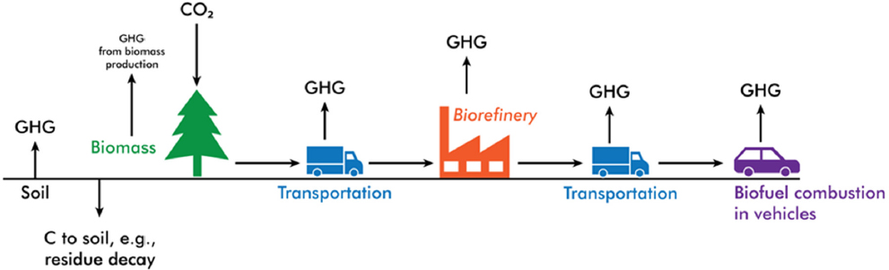
Different methods of evaluating carbon flows for short-rotation crops and long-rotation woody biomass are assessed and discussed in this section. Changes in soil carbon caused by LUC can generate significant GHG emissions; the soil carbon section discusses different models and methods to estimate soil carbon change and the challenges in modeling and data collection. GHG emissions associated with growing and harvesting are discussed in Chapter 9. Emissions are generated during the process of combustion of biofuels in a vehicle and during the process of conversion of feedstock (e.g., corn) to fuel in a refinery and its transportation to the consumer. These emissions can be referred to as biogenic carbon, contemporary carbon, or organic carbon. In contrast, the carbon in petroleum, natural gas, and coal is referred to as fossil carbon.

Biogenic CO₂ emissions are the release of the carbon embodied in the feedstock that was removed from the atmosphere through the process of photosynthesis and stored in the biomass. These emissions are returned to the atmosphere during the process of conversion of the feedstock to biofuel in a refinery and through combustion of biofuel in a vehicle. These biogenic emissions are sometimes excluded from the estimation of the GHG intensity of corn ethanol (Wang et al., 2012). This approach is controversial, and some studies accounted for these biogenic emissions (during conversion and combustion) to determine the extent to which they are offset through sequestration during biomass regrowth. The feedstock for biofuels from annually harvested agricultural crops has sometimes been treated as carbon neutral in that the annual biogenic carbon uptake by the feedstock from the atmosphere is considered to offset the emissions released during conversion and combustion of the biofuel. It is important to note that, based on this reasoning, only the biogenic carbon emissions embodied in the feedstock and released during its production and consumption as fuel are considered carbon neutral; it is not intended to imply carbon neutrality of the life-cycle emissions (De Kleine et al., 2016). This approach of treating all biogenic carbon as carbon neutral ignores more potent GHG emissions, particularly methane (CH₄), that may be generated in the process of conversion and release of biological carbon. Thus, with different global warming potentials for different forms of carbon, the fuels with non-CO₂ GHG emissions cannot be considered carbon neutral. This is one of the core reasons in the argument against assuming carbon neutrality of biogenic carbon, and there are other reasons such as the impacts of land use and temporal aspects associated with long-rotation feedstocks (Fargione et al., 2008; Lan et al., 2021; Searchinger et al., 2008; Wiloso et al., 2016).

Biogenic Emissions from Annually Harvested Feedstocks

The treatment of biogenic CO₂ emissions from agricultural feedstocks, specifically food crops, converted to biofuels as carbon neutral has been questioned by DeCicco (2016), Searchinger (2010), Searchinger et al. (2009), and others (Fargione et al., 2008; Lan et al., 2021; Searchinger et al., 2008; Wiloso et al., 2016). When food crops, such as corn and soybeans, are used to produce biofuels, two things happen in order to meet the demand for biofuel. First, there is some diversion of the crop from food/feed use to

produce biofuels. Second, this raises crop prices (given a fixed demand for food/feed) and creates incentives to bring additional land to be planted under this crop to produce feedstock for the biofuel. Thus the total feedstock used for biofuel production is partly coming from the existing production and partly from new (additional) production of feedstock.

Searchinger (2009) suggests that “biomass should receive credit to the extent that its use results in additional carbon from enhanced plant growth or from the use of residues or biowastes.” In other words, the carbon uptake by the crop that would have been produced anyway for use as food/feed should not be used as an offset for the carbon emissions during production and combustion of the biofuel. The additional carbon may be generated from the increase of biomass uptake due to changes in land management or from the utilization of biomass that would otherwise emit GHG emissions through rapid decomposition (Searchinger, 2009). DeCicco et al. (2016) use an analysis of direct carbon exchanges by comparing only the additional biogenic carbon emissions uptake during the production of the feedstock directly converted to biofuel and the biogenic emissions released during the production and combustion of the biofuel. DeCicco et al. (2016) mentioned their work as a narrow analysis that examines carbon neutrality by evaluating the extent to which feedstock CO₂ uptake offsets biogenic CO₂ emissions from fuel combustion.

De Kleine et al. (2017) have argued that for crops being grown and harvested annually, all carbon taken up by the crop, whether the crop is used for food, feed, or fuel will be returned to the atmosphere within a year or in a short period. This contemporary carbon, when released by a biorefinery or vehicle, should not be considered as net addition of carbon to the atmosphere. They explained that biofuel production leads to an exactly equal increase in net ecosystem production; therefore a 100 percent biogenic carbon offset should be applied. Net ecosystem production was used by DeCicco et al. (2016) to estimate the additional carbon, which is a portion of carbon taken up by biomass that becomes material available for local sequestration or other disposition. In response to this argument, DeCicco (2017) pointed out the need for careful analysis to circumscribe the temporal and spatial scope for any net ecosystem production increase instead of assuming that net ecosystem production increases occur somewhere and justify the full biogenic carbon offsets. Furthermore, the use of biomass for one purpose affects the production of biomass for other purposes (plant growth), so there can be an opportunity cost from reducing biomass productivity. The assessment of carbon emissions of non-food crops used as feedstocks for biofuels may be considered to depend on the alternative use of the land on which they are grown. Future research should clarify how changes in carbon stock (including soil carbon change) are being considered in assessing changes in net ecosystem production (DeCicco and Schlesinger, 2018; Field et al., 2020, 2021; Haberl et al., 2012; Kalt et al., 2019; Khanna et al., 2020; Searchinger, 2012; Searchinger et al., 2018).

Different frameworks exist, and one of them was developed by EPA for biogenic CO₂ emissions from stationary sources. This framework “assesses the extent to which the production, processing, and use of biofuels results in a net atmospheric contribution of biogenic carbon emissions”. This assessment framework does not “include a full LCA, which would take into account all upstream and downstream GHG emissions and sequestration related to feedstock production and use, including from all fossil fuel inputs used, for example, to power machinery used to harvest and transport biogenic feedstocks.” The framework mentions the key decisions for biogenic CO₂ flux assessment, including the choice of baseline, temporal and geospatial scales, and feedstock categories. In this framework, the baseline approach is used to evaluate the landscape emissions associated with the feedstock growth, potential leakage, biogenic emissions that would have occurred on the feedstock landscape without the use of biogenic feedstock, and changes in land use or land management. The EPA framework presents two baseline approaches. The first is the Reference Point Baseline approach that measures the net change in carbon between two points in time. The second approach is the Anticipated Baseline approach, where the carbon stocks in a baseline scenario that "establishes historic or simulates future anticipated biogenic feedstock use and related environmental and socioeconomic conditions and impacts along a specified time scale" is compared with an "alternative scenario of changed (e.g., increased or decreased) biogenic feedstock demand.” The EPA framework suggests no preferences between the two approaches. The Reference Baseline approach has several limitations. First, it attributes all of the changes in carbon stocks in the after–biofuel production scenario to the level of biofuel production relative to the start year; this disregards other factors that could have changed over time, such

as, weather, market conditions and technology that affect carbon stocks. Second, the time period chosen as the reference point can influence the magnitude of biogenic emissions that are considered additional. The limitation of the Anticipated Baseline approach is the uncertainty associated with assumptions for future scenarios. These future anticipated baselines need to be developed using some modeling or analytical approaches, such as dynamic modeling or extrapolation of historical trends, which bring in different kinds of uncertainty (EPA, 2014).

Biogenic Emissions from Long Rotation Feedstocks

Demand for long-rotation feedstock such as forest feedstocks for bioenergy could be met by some combination of increasing intensity of forest harvest; diverting biomass from other uses such as pulp, timber, and mill residues; and by planting more land under forests. Increasing the intensity of forest harvesting will reduce the stock of carbon on existing forestland and create a carbon debt. Diversion of biomass from other uses, such as pulp and timber that can be stored for forest carbon, can also create a carbon debt (Fargione et al., 2008).

Researchers use a variety of methods to estimate carbon debt in long-rotation feedstocks. Two commonly used approaches are stand-level and landscape-level assessments, and a third less-common approach is the dynamic landscape-level assessment, which are all described below. These approaches are points on the LCA spatial spectrum, as defined in the goal and scope definition phase, that can range from a forest stand to global forested land. A forest stand is “the fraction of a landscape belonging to one age class” (Berndes et al., 2013; Peñaloza et al., 2019) while a forest landscape is an area with different age classes. Stand-level assessment models the forest system as a single stand of trees or an increasing stand of trees. Therefore stand-level carbon accounting can show the carbon dynamics of sequential events such as site preparation, plantation, thinning, tree growth, and final harvest. The starting point of analysis strongly affects the results of stand-level assessment (Cowie et al., 2021). Landscape-level assessment considers a fixed landscape of several stands that are being managed jointly to meet the demand for forest biomass in a continuous manner, or a region in which land can move in and out of forest production. With a single stand scale of accounting, increase in the harvest of trees for bioenergy will result in a carbon debt and then a dividend. This is because at a stand level, trees can take many years to grow back after harvest; there is a time interval between carbon release and re-absorption of that carbon from the atmosphere, which can temporarily increase GHG emissions in the atmosphere. As a result forest bioenergy may not necessarily be carbon neutral or it may only be carbon neutral over longer time frames (Cherubini et al., 2011; McKechnie et al., 2011). The magnitude of this debt may depend on the counterfactual level of carbon stock that is considered to prevail in the absence of the demand for bioenergy. This could be one where the forest is being cut for timber only, or it could be a forest that is never harvested; the carbon debt created by cutting a natural forest is larger than with cutting a plantation forest.

One alternative to the stand-level view of forest management is the landscape view of the forest that recognizes a forest that is being managed in a way to generate biomass continuously to feed an industrial operation. In this case if the demand for bioenergy leads to more intensive harvesting then the carbon stock in the landscape could decrease, but the carbon debt created would be spread out across the landscape and be recovered over a shorter time frame (as in Dwivedi et al., 2016). In this case the landscape is managed in an integrated way like a plantation that is part of a bioenergy supply chain and the whole fuel shed is considered together when examining the carbon balance (Jonker et al., 2014).

A third approach is one that allows the size of the landscape to change dynamically in the scenario with forest bioenergy use compared to the baseline with no harvesting of the forest for bioenergy. The dynamic landscape view incorporates market-driven effects that arise when the demand for bioenergy affects the returns to land and creates incentives for LUC as well as for changing forest management practices. In this view, biogenic carbon accounting involves accounting not only for changes in carbon stock in standing biomass but also for changes in carbon stock due to changes in land use as land moves in and out of forestry. It also accounts for changes in carbon stock as forest biomass is diverted from wood products, which provide long-term storage for carbon, to bioenergy.

The differences between stand-level and landscape-level approaches have been widely discussed in literature (Cintas et al., 2016; Cowie et al., 2021; Peñaloza et al., 2019). Jonker et al. demonstrated how stand-level and landscape-level approaches yield different carbon debts. Using the stand-level approach, the study estimated the carbon debt based on the forest carbon stock changes of stands at the same age. Using the landscape-level approach, they estimated the carbon debt as the average carbon debt of uneven-aged trees (in this study, 0–25 years for low management intensity and 0–20 years for high management intensity) (Jonker et al., 2014). Stand-level and landscape-level approaches answer different questions (Cowie et al., 2021). Stand-level assessment provides in-depth understandings of growth patterns and interactions between different carbon pools in the forests (Cowie et al., 2021). Landscape-level assessment better represents the dynamics of the forest system managed at a landscape level in which fluctuations observed at the stand level are evened out (Cowie et al., 2013). It can consider changes in forest management in response to retrospective or anticipated bioenergy demand, as well as natural disturbance such as fire. Previous studies suggest stand-level assessment may be useful when one specific forest stand can be traced for a forest product (Peñaloza et al., 2019) or when the purpose is to inform forest management; while landscape-level assessment is appropriate for assessing the large-scale impacts of bioenergy policy (Cowie et al., 2021).

Forest Bioenergy

In the case of forest bioenergy it is important to integrate both LCA of supply chain emissions during the production of the feedstock as well as biogenic carbon due to changes in forest carbon stocks (which could be biogenic carbon emissions or sinks, depending on the net forest carbon stock changes) to provide a complete assessment. This accounting is needed because life-cycle related carbon emissions from bioenergy production can be expected to be accompanied by changes in forest management practices that will affect biogenic carbon stocks, for example by affecting the age at which trees are harvested, the intensity with which forests are managed, the species that are planted, the collection of residues, and a change in land use between forestland and cropland. Life-cycle accounting of the CI of using pulpwood for bioenergy needs to consider the forgone sequestration of biogenic carbon in forest products due to the diversion of biomass from forest products to bioenergy. Collection of logging residues for bioenergy will involve emissions in the collection and transportation of biomass but lead to avoided biogenic carbon emissions from gradual decay of forest biomass. This practice will lead to biogenic emissions during combustion of the residues but can displace fossil emissions from generating an equivalent amount of energy. Since changes in land use and in the production of forest products in bioenergy scenarios are likely to be induced by market price changes caused by the increased demand for bioenergy, including their carbon implications requires a dynamic landscape-based accounting approach.

In some methods of accounting, it is necessary to cumulate the changes in biogenic carbon over a specified time horizon and add them to the life-cycle emissions over the same horizon. This approach requires specifying a time frame over which to cumulate the negative and positive changes in biogenic carbon over time to estimate the total carbon impact of increased demand for bioenergy (McKechnie et al., 2011). Typically, for a forestland, carbon stocks could decrease in the near term after harvest and then grow in the future with forest regrowth. The estimated overall impact of bioenergy demand will depend on the time horizon used to account for the total effect. A short time horizon for cumulating changes will ignore longer term impacts and could under- or over-estimate the carbon impacts of forest bioenergy. Studies differ in the time horizon used for cumulating the impact of a demand for forest bioenergy on forest carbon stocks. Jonker et al. (2014) use a 75-year horizon as the time frame while McKechnie et al. (2011) use a 100-year horizon; these studies provide no scientific criteria to choose the justification for the choice of time horizon. Thus, using different time frames may be appropriate to explore the sensitivity of results. The magnitude of the carbon savings with using forest biomass for bioenergy relative to the baseline increases as the length of the time horizon increases.

Sometimes woody biomass is assumed to be carbon neutral if it is harvested from a forest with stable or increasing carbon stock, which is questionable if the life-cycle GHG emissions and all biogenic

carbon flows are not considered and compared with a realistic counterfactual scenario (Cowie et al., 2021). This carbon neutral assumption is often used as a basis for ignoring and not reporting biogenic carbon. However, whether and how long the biogenic carbon can be fully refilled by growth or re-growth of forest depends on many factors such as the temporal and geospatial scales of the carbon analysis and the impacts of biofuel production on forest management, as discussed previously. Optimistic assumptions (Giuntoli et al., 2020) of forest management practices in counterfactual scenarios assumed in the literature may overstate the carbon savings associated with forest biomass. Stand-level analysis is more often used in LCAs for forest bioenergy, given its capacity to investigate sequential forest management activities, growth patterns, and different carbon pools. Landscape-level analysis allows for exploring forest dynamics, especially the changes in forest management and carbon stocks in response to biofuel demand (Cowie et al., 2021). The landscape-level analysis may be more challenging given the additional data needs of forest carbon stocks. Historical data available from the U.S. Forest Service could be used as a reference to understand the potential impacts of using woody biomass for biofuel production.

In sum, different biogenic carbon accounting methods exist but there is no method widely agreed upon (Brandão et al., 2013). This committee does not endorse any biogenic accounting method discussed in this section. Biogenic carbon has been included in some studies with a simultaneous consideration of carbon uptake and release, while some other studies exclude biogenic carbon.

For long-rotation woody biomass, stand-level and landscape-level approaches have been used; both methods consider forest carbon stock changes but differ in the temporal and spatial scale of accounting for these changes.

Soil Carbon

LUC, land management, and land management change (e.g., reducing tillage frequency, applying manure as a soil amendment) can alter soil carbon (NASEM, 2019). These changes and corresponding GHG emissions (or carbon sequestration) can be accounted for in LCA. For example, if a biofuel is to be made from an energy grass feedstock that is planted on land that was previously planted in corn, the changes in soil carbon per unit land area could be multiplied by the amount of land previously in corn that is now planted in energy grasses, but there would also be changes in land use elsewhere due to market-mediated effects. More broadly, the results of LUC models that predict the amounts, types, and locations of land that would be used for feedstock production can be used in conjunction with soil organic carbon (SOC) modeling results to estimate soil carbon stock changes that would accompany widespread LUC.

There are some efforts (Ledo et al., 2019) to gather and distribute the data for soil carbon changes (Xu et al., 2019). It is common to estimate soil carbon changes. One way of doing this is to use the Intergovernmental Panel on Climate Change (IPCC) emission factors. The simplest approach the IPCC offers is use of Tier 1 emission factors, which allows for SOC change estimation even in the absence of site-specific data. In the 2019 Refinement to the 2006 IPCC Guidelines for Natural Greenhouse Gas Inventories,⁵ IPCC puts forward reference SOC stocks for six different soil types in 10 climate regions. These values are accompanied by an uncertainty value that in some cases is the 95 percent confidence interval but may also be 90 percent of the mean value when limited data are available. If more data are available (e.g., country--

___________________

⁵ See http://www.ipcc-nggip.iges.or.jp/.

specific data on tillage practices or reference soil carbon stock) IPCC defines two additional levels of SOC calculations, Tier 2 and Tier 3.

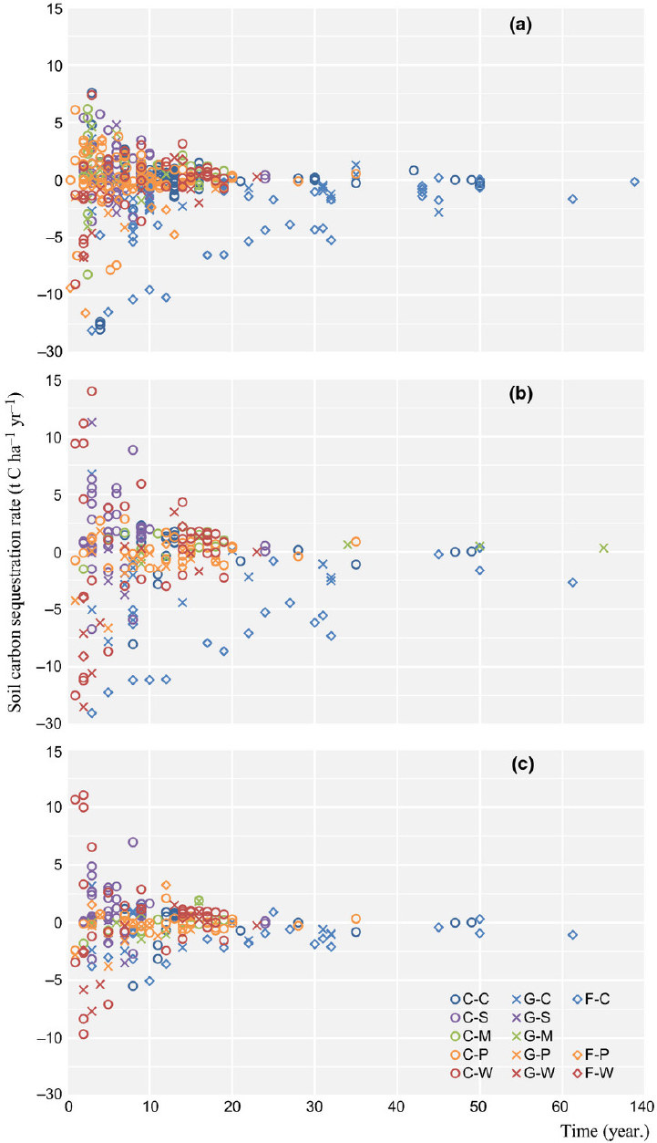
Another approach is to use a soil carbon model such as DAYCENT (Colorado State University, n.d.) or CENTURY (Parton, 1996) although many other models exist (e.g., MEMS [Zhang et al., 2021]) or to build a model for specific use in a study. There are many parameters involved in SOC modeling. Documenting them transparently can improve the LCA community’s ability to interpret the defensibility of the SOC modeling approach. For example, the choice of soil depth can influence results. Historically (see EPA, 2010), a soil depth of 30 cm was often used, but SOC changes further below the surface (e.g., 100 cm) can be notable, particularly for deep-rooted energy crops (Qin et al., 2014, see Figure 6-2).

Modeling results that choose a final year soon after a disruption to historical land use may report SOC changes that are very large and not reflective of long-term trends. On the other hand, if land use, cover, or management practices change frequently, the soil carbon model will not reach equilibrium. In that case, choosing the starting and final SOC values can be challenging. One notable challenge in using soil carbon models is determining the appropriate land use history. This can be particularly challenging for land that may be idled in some years and planted in crops in others. Some studies show that SOC modeling results can be insensitive to assumptions about land use history (Emery et al., 2017). However, this is not true in every instance, and transparency in the choice of land use history, and other SOC modeling parameters, is important. Some have argued that using SOC modeling approaches that assume too detailed of an approach to land use history could introduce a false sense of confidence in results and that a more general approach is more appropriate. Further study supported by SOC data is needed to support a harmonized approach to addressing land use history modeling, particularly for marginal lands or cropland-pasture that varies in how it is used.

Recently, the permanence of any soil carbon change has come into question for at least two main reasons. Even if land management practices do not change, climate change can “undo” SOC stock gains. Permanence issues have been raised in multiple literature reports (Dynarski et al., 2020; Leifeld and Keel, 2022). Accordingly, permanence needs to be raised as a methodological issue that arises in biofuel LCA. First, economic or political conditions may change, which may affect land use. For example, soil carbon stored due to conversion of row cropland to perennial species, such as with the Conservation Reserve Program of the USDA Farm Service Agency, may be lost when land is returned to production. Second, given the influence of climate on SOC (Hicks Pries et al., 2017), future SOC modeling efforts may need to address the changing climate.

Given the uncertainty arising in SOC modeling, reporting of uncertainty assists the community in interpreting SOC modeling results that are used in LCA.

Overall, more data are needed to inform both high-level approaches such as those in the IPCC Tier 1 methodology, to inform the parameters used in SOC modeling, and to provide ground truth to validate SOC modeling results. It should be noted that IPCC Tier 1 methodology may have limited value for assessing SOC effects of dedicated perennial bioenergy crops, which could be treated as generic “managed grassland” or “managed forest,” which would not account for the high productivity of these purposefully-selected crops. These data could be collected from emerging, remote-sensing based methods that may be more cost effective and rapid than conventional sampling methods.

In sum, changes in SOC can be a significant contributor to the life-cycle GHG emissions of a biofuel. SOC modeling results are sensitive to parameters including soil depth and land use history. The permanence of modeled SOC changes is uncertain given climate change and other factors that could include market drivers or policy changes that would influence land use. Researchers have varying views on the level of detail that is appropriate in modeling SOC, in particular for land use history. Despite efforts to collect additional data, many data and knowledge gaps remain regarding SOC changes for land with varying land use histories used to grow different biofuel feedstocks. These data gaps impede calibration and validation of soil carbon models.

INDICATORS, OTHER CLIMATE FORCERS, AND TIMING OF EMISSIONS

Fuels lead to the emission and uptake of CO₂ (biofuel) and other GHGs in every life-cycle stage. These emissions and uptakes must then be aggregated into a common unit so that the climate change impact of different fuels can be compared. To aggregate different GHG emissions into a common unit, namely CO₂ equivalent (CO₂e), metrics expressing the relative contribution of GHGs to climate change are needed. Since its publication in the First Assessment Report of the IPCC in 1990 (IPCC, 1990) and its adoption for the application of the Kyoto Protocol, global warming potential (GWP)⁶ calculated for a 100-year time horizon (GWP₁₀₀) established itself as the most commonly used metric in LCA (Levasseur et al., 2016a).

GWP is the cumulative radiative forcing caused by a unit-mass of GHG released to the atmosphere, integrated over a given time horizon, relative to that of a unit-mass of CO₂. However, as stated by the authors of the First Assessment Report: “It must be stressed that there is no universally accepted methodology for combining all the relevant factors into a single global warming potential for greenhouse gas emissions. A simple approach (GWP) has been adopted here to illustrate the difficulties inherent in the concept” (IPCC, 1990). Despite this warning, the use of GWP for a 100-year time horizon in LCA has rarely been challenged. In its Fifth Assessment Report, the IPCC reminds that “the most appropriate metric will depend on which aspects of climate change are most important to a particular application, and different climate policy goals may lead to different conclusions about what is the most suitable metric with which to implement that policy” (Myhre et al., 2013).

Since the IPCC First Assessment Report, the science regarding climate metrics has evolved, and many other metrics have been proposed to compare the climate impact of different GHGs. For instance, in its Fifth Assessment Report (Myhre et al., 2013), IPCC proposes and discusses the use of global temperature change potential (GTP) for 20-, 50-, and 100-year time horizons in addition to GWP for 20- and 100-year time horizons. GTP is defined as the instantaneous global temperature change caused by a unit-mass of GHG released to the atmosphere a given number of years following the emission corresponding to the time horizon selected, relative to that of a unit-mass of CO₂ (Shine et al., 2005). Additional metrics, such as global precipitation potential (Shine et al., 2015), are presented in the very recent IPCC Sixth Assessment Report (Forster et al., 2021).

Metrics vary according to the element of the cause–effect chain that it quantifies (e.g., radiative forcing for GWP, temperature change for GTP or precipitation change for global precipitation potential), the time horizon selected, and its cumulative or instantaneous nature. An instantaneous metric quantifies the change at a particular time after the emission, expressing the effect of the emission persisting after a

___________________

⁶ A measure of how much energy the emissions of 1 ton of a gas will absorb over a given period, relative to the emissions of 1 ton of CO₂.

given time horizon. A cumulative metric integrates the impact over the selected time horizon following the emission, that is, it expresses the total effect from the time of the emission up to the given time horizon. Any metric can be presented as an absolute value, or as a relative value, dividing the absolute value by the equivalent value for CO₂ (Forster et al., 2021). Instantaneous metrics could be deemed more appropriate if the goal is to not exceed a fixed target at a specific time, while cumulative metrics could better suit the need to reduce the overall damage when the impact depends on how long the change occurs for (Forster et al., 2021). The selection of a time horizon can also be driven by the types of impact to be captured by the metric. On the one hand, metrics addressing shorter-term climate change are more appropriate to capture impacts affected by the rate of change such as the adaptation of species to changing habitat, heat stress, or extreme weather events. On the other hand, metrics addressing long-term climate change are more suitable for impacts associated to sea level rise or coral bleaching, among others (Levasseur et al., 2016a).

In its Sixth Assessment Report, IPCC also discusses new emission metric approaches, such as GWP*⁷ (Cain et al., 2019; Smith et al., 2021) and combined global temperature change potential (Collins et al., 2020), that have been developed to better account for the different physical behaviors of short- and long-lived GHGs. They found that these new approaches can improve the evaluation of the contribution to global warming of different GHGs within a cumulative emission framework, as pulse-based emission metrics (e.g., GWP, GTP) do not represent accurately the effect of sustained short-lived GHG emissions (Forster et al., 2021). The combined global temperature change potential values are published in the IPCC Sixth Assessment Report and are to be applied to a change in emission rate rather than a change in emission amount, as it has been designed for cumulative emission frameworks such as national-level inventories, which is different from the LCA framework.

From 2014 to 2016, the Life Cycle Initiative, hosted by the United Nations Environment Programme (UNEP), led an international initiative aiming at developing consensus-based metrics for use in LCA for climate change. A task force composed of researchers from both the climate metric and LCA fields performed a critical analysis of the most recent scientific findings and developed recommendations (Cherubini et al., 2016; Levasseur et al., 2016b). This was followed by a consensus-finding workshop (Jolliet et al., 2017; Levasseur et al., 2016a). Indicators were evaluated according to their environmental relevance, that is their capacity to cover the broad spectrum of relevant long- and short-term impacts, as well as reliability. The recommendation from this international consensus-finding workshop is to use two different indicators in parallel: GWP for 100 years (GWP₁₀₀) for shorter-term impacts, and GTP for 100 years for long-term impacts, including climate–carbon feedbacks for both.

For very short-term impacts, another recommendation from the international consensus-finding workshop is to perform a sensitivity analysis using GWP for 20 years, including emissions from near-term climate forcers. Near-term climate forcers (CO₂, NO_x, SO_x, volatile organic compounds, black carbon, and organic carbon) affect the climate through different physical and chemical mechanisms (e.g., changes in methane lifetime or cloud cover). These pollutants have lifetimes in the atmosphere of days to weeks, which is too short to allow them becoming well mixed in the atmosphere, leading to strong spatial and temporal heterogeneities (Myhre et al., 2013). Therefore, their global warming impact highly depends on the region of emissions and are very short-term, which makes their aggregation to a CO₂e unit challenging (Levasseur et al., 2016a). This regional variability increases uncertainties associated with emission metrics for near-term climate forcers. However, their contribution to the rate of temperature increase in the short-term has been shown to be important (Allen et al., 2020; Fuglestvedt et al., 2008).

Another issue related to the evaluation of the contribution of CO₂ and other GHGs to global warming is the consideration of the timing of emissions and uptakes. Some emissions and uptakes within the life cycle of biofuels might occur several years or decades before or after the fuel is produced and used. The two most discussed cases in the literature regard carbon uptake by growing biomass, which can occur over several years after harvesting for forest or long-rotation crops (Lamers and Junginger, 2013; McKechnie et

___________________

⁷ GWP* is an alternative application of GWPs where the CO₂-equivalence of short-lived climate pollutant emissions is predominantly determined by changes in their emission rate. See https://iopscience.iop.org/article/10.1088/1748-9326/ab6d7e.

al., 2011; Zanchi et al., 2012), and upfront LUC emissions for short-rotation crops, which are usually amortized over several years of biomass production (Fargione et al., 2008; Levasseur et al., 2010). Upfront LUC emissions, incurred immediately but occurring both in the short- and long-term, and delayed carbon uptakes both lead to a so-called carbon debt.

Using common accounting approaches, a given CO₂ emission is considered compensated by the uptake of an equivalent amount of CO₂, no matter when they occur. However, if the emission occurs several years before the uptake, the CO₂ released will contribute to global warming on the short-term, and the time required to reach a net-zero warming effect can be several decades or centuries (Levasseur et al., 2012). Moreover, biogenic carbon emissions from biofuel combustion are usually disregarded in LCA, as they are systematically considered compensated by equivalent uptakes, which could lead to potential accounting errors (Searchinger et al., 2009). Given the urgency of climate change and the ambitious binding targets for GHG emission reduction set by climate policies such as the Paris Agreement (i.e., net zero CO₂ emissions in 2050), the increase in GHG emissions in the short-term could be an issue even if they are compensated by equivalent uptakes later on.

Different approaches have been proposed to address the timing issue of GHGs in LCA. Some of them are applicable to very specific cases. For instance, the PAS 2050 carbon footprint standard (British Standards Institute, 2008) and the EU International Life Cycle Data System (ILCD) Handbook (European Commission, 2010) proposed methods to account for the climate benefits associated with temporary carbon storage in long-lived products. O’Hare et al. (2009) and Kendall et al. (2009) proposed two different approaches to amortize upfront LUC emissions for short-rotation crops, while considering their contribution on global warming. Cherubini et al. (2011) proposed a new metric to assess biofuel combustion emissions while accounting for the delay of carbon uptake, depending on the biomass rotation period. Levasseur et al. (2010) proposed the broader dynamic LCA approach in order to account for the timing of every GHG emission and uptake in LCA. The method develops a temporally differentiated inventory, then calculates associated radiative forcing over time based on the models used to calculate GWP values. A similar approach has been proposed and applied to the assessment of bioenergy systems, using the temperature change as an indicator instead of radiative forcing (Ericsson et al., 2013).

The use of any of these approaches implies the selection of a time horizon beyond which global warming impacts are disregarded. Therefore, an emission occurring the first year will lead to a higher impact than an emission occurring 25 years later, as this second emission will contribute to global warming for a period of 75 years instead of 100 years, given that a 100-year time horizon is selected. For methods proposing new metrics for specific cases (e.g., Cherubini et al., 2011; Kendall et al., 2009; O’Hare et al., 2009), the time horizon is fixed by the developers. In contrast, methods based on the dynamic LCA approach provide time-dependent impacts (radiative forcing or temperature change), and it is up to the decision-maker to select one or more time horizons for the comparison of fuels. Dynamic LCA results are more complex to understand for non-experts compared to approaches proposing specific metrics, but they allow decision-makers to compare the global warming contribution of different fuels on the short-, mid-, and long-terms as different time horizon can be selected for the analysis.

Different metrics capture different climate change impacts, depending on their characteristics (e.g., cumulative or instantaneous, time horizon). It is recognized that the most appropriate metric depends on which aspects of climate change are most important to a particular application. Some biofuel pathways lead to a so-called carbon debt, increasing global warming impacts in the short-term. Given the urgency of climate change and the ambitious binding targets for GHG emission reduction set by climate policies such as the Paris Agreement (i.e., net zero CO₂ emissions in 2050), the increase in GHG emissions in the short-term could be an issue even if they are compensated by equivalent uptakes later on. The most recent research, including the recently published IPCC Sixth Assessment Report, present different metrics to aggre-

gate GHG emissions into a single unit. Different metrics can be used depending on the context of application (e.g., national-level inventories, LCA), and the type of climate change impacts to address (e.g., extreme weather events or species adaptation related to the short-term temperature peak, sea-level rise associated with the longer-term stabilization temperature). Some studies reviewed different GHG metrics, such as Brandão et al. (2019). There is a clear consensus in the literature that the sole use of GWP₁₀₀ does not capture the full range of climate change impacts.

Low-carbon fuels could also affect the climate through mechanisms other than GHG and near-term climate forcer emissions. The production of biomass often leads to land cover changes (e.g., transformation of natural lands to crops, forest harvesting), which could then affect the albedo, i.e., the proportion of solar radiation reflected by the surface. Researchers have estimated the potential warming or cooling effect of albedo modifications due to different land cover changes for bioenergy production (Cai et al., 2016; Cherubini et al., 2012; Darvin et al., 2014; Holtsmark, 2015). Some have shown that, in some cases, the order of magnitude of the climate effect due to albedo modifications can be as high as that of associated carbon stock changes (Betts, 2000; Jones et al., 2013). This is the case for harvesting forests at high latitudes because of the reflectivity of snow cover in the winter (Bernier et al., 2011). Although potentially very important, climate impacts from albedo changes are difficult to quantify in LCA because they are site-specific and rely on solar irradiance measurements (Sieber et al., 2019). Some approaches have been proposed by researchers for their integration in LCA, but they have not yet been implemented (Muñoz et al., 2010; Sieber et al., 2020).

Biofuels could affect the climate through mechanisms such as modifications in surface albedo due to land cover changes. Although potentially very important, climate impacts from changes in albedo, evapotranspiration, or other biogeophysical changes are difficult to quantify in LCA because they are site-specific and rely on solar irradiance measurements. Researchers have proposed different approaches to account for the timing of GHG emissions and uptakes. However, all these approaches rely on the subjective choice of a time horizon beyond which impacts are disregarded. There is currently no consensus in the literature regarding the valuation of delayed emissions in LCA.

VEHICLE–FUEL COMBINATIONS AND EFFICIENCIES

Life-cycle GHG emissions of transportation fuels can be compared on a per-unit-energy basis (e.g., emissions could be measured per MJ of a fuel’s energy), but such a comparison can be incomplete or misleading without also considering how much energy is needed to propel a vehicle with each type of fuel as well as how much energy is required, and how much emissions are created in the production and maintenance of each type of vehicle. Efficiency and production emissions can vary widely both within and across vehicle fuel type technologies, making fair comparisons with single point estimates challenging. This section discusses issues specific to the vehicles that convert transportation fuels into transportation services.

To compare emissions from transportation fuels, rather than using an energy-based functional unit, a more meaningful functional unit might be based on the transportation services delivered. Common functional units for passenger transportation in the United States are vehicle-mile or passenger-mile, and a common functional unit for transportation of goods in the United States is ton-mile. Using a functional unit based on transportation services provided requires knowing or estimating the efficiency of the vehicle and, in some cases, the number of passengers or weight of cargo transported. The service-based functional unit could be reported in addition to an energy-based functional unit.

The life-cycle implications of transportation fuels depend on the vehicle efficiency as well as emissions associated with production, maintenance, and disposal of vehicles.

The efficiency of the vehicle that will use the fuel is typically unknown to the fuel producer and heterogeneous across fuel customers. The CA-LCFS policy handles this by introducing energy efficiency ratios. This section will first discuss issues of LCA of transportation fuels and then discuss how energy efficiency ratios are used in CA-LCFS policy.

Efficiency

Vehicle efficiency can vary widely within and across fuel types, as well as across driving conditions; individual vehicles also have variations based on the level of maintenance (e.g., tire pressure). Models that use a single “representative” vehicle to represent each fuel type can mask this heterogeneity. This section summarizes and quantifies the efficiency of vehicles available today that use each fuel type and summarizes how much the efficiency of each fuel can change depending on conditions that vary regionally and across drivers, such as weather, terrain, driving style, regional energy sources, and other factors.

Variation in Vehicle Design

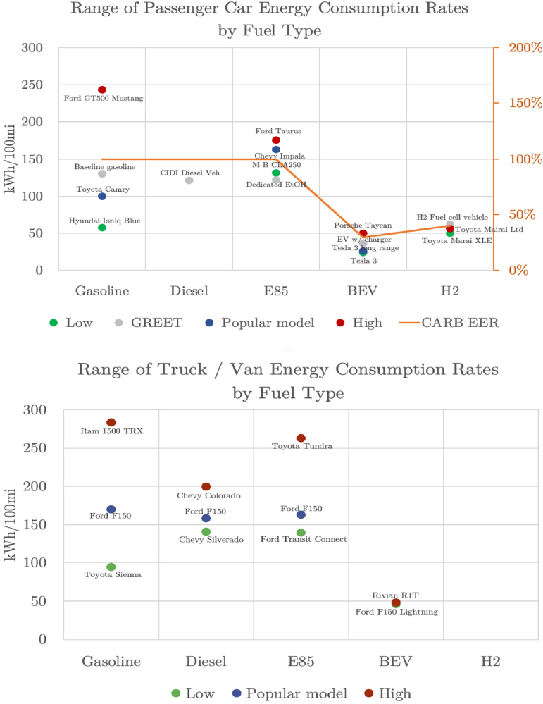
Figure 6-3 summarizes the energy consumption rates of vehicles by fuel type. Energy consumption rates (kWh/mile) are used here rather than efficiency (mile/kWh) because emissions implications are proportional to consumption rates (and inversely proportional to efficiency) (Larrick and Soll, 2008). Figure 6-3 shows a range of new vehicles available for sale today, with efficiency values taken from fueleconomy.gov, including (1) the least efficient mass-market vehicle for each fuel type (excluding low-volume luxury and sport models, such as Rolls-Royce and Lamborghini designs); (2) the most efficient mass-market vehicle for each fuel type; and (3) one of the most popular vehicles for each fuel type sold in the United States. In addition, for passenger cars the figures include the efficiency value used in GREET. There are no mass-market hydrogen vehicles today, so the three available (low-volume) models are used to establish the range. All energy values are converted to kWh, and consumption rates are reported in kWh per 100 miles. Plug-in hybrid electric vehicles (PHEVs), which use a combination of grid electricity and gasoline, are not shown, and E85 vehicles represent the efficiency of flex fuel vehicles when operating on E85 (with the exception of the GREET data point, which represents a dedicated E85 vehicle). For comparison, the energy efficiency ratios (inverted to map to relative consumption rates) used in CA-LCFS are also plotted on a secondary axis.

Variation in Use Conditions

The energy consumption rates presented previously are based on driving cycles performed in a laboratory, where each vehicle is placed on a dynamometer (like a treadmill for a vehicle), driven to follow a prescribed sequence of vehicle speeds, and monitored to assess fuel consumption and emissions. The advantage of such a test is standardization—all vehicles can be compared in the same conditions, ensuring an apples-to-apples comparison. However, such a test masks important variation in real-world effects that can differ across fuel types.

Real-world driving conditions, including speed, acceleration, frequency and duration of stops, driving distance, precipitation, temperature, humidity, and other factors affect the efficiency of all vehicles, but the effect can be larger for some fuel types than others (Karabasoglu et al., 2013).

Climate and weather conditions also affect vehicle efficiency for different fuel types differently. Cold weather generally makes all vehicles less efficient, but it has a larger effect on electric vehicles (EVs) than gasoline vehicles. Gasoline vehicles are less efficient when cold for a variety of reasons, including increased viscosity of engine lubricants, but gasoline vehicles can use waste heat from the engine to heat the passenger cabin. In contrast, EVs are less efficient when cold both because batteries are less efficient when it is cold and because energy from the battery must be used to heat the cabin. Figure 6-4 shows energy consumption rates for an internal combustion engine vehicle (ICEV), hybrid electric vehicle (HEV), PHEV and battery electric vehicle (BEV) normalized to fair weather efficiency. Electrified vehicle efficiency is more sensitive to ambient temperature than gasoline vehicle efficiency. Note that Figure 6-4 is shown relative to fair-weather efficiency. In absolute terms, electrified vehicles are typically more efficient.

Variation of fuel consumption rates can be larger within fuel type than across fuel type, especially for gasoline, for which fuel consumption rates vary by more than a factor of 4. Some of this variation is due to vehicle class (e.g.: sports car vs. compact car), but there is substantial variation within vehicle class.

Figure 6-5 shows the implications of these differences in efficiency for energy consumption in different parts of the United States, based on temperature data across a typical year. The same vehicle with the same driving patterns consumes about 20 percent more energy in regions with extreme heat and cold than in regions with consistently mild weather.

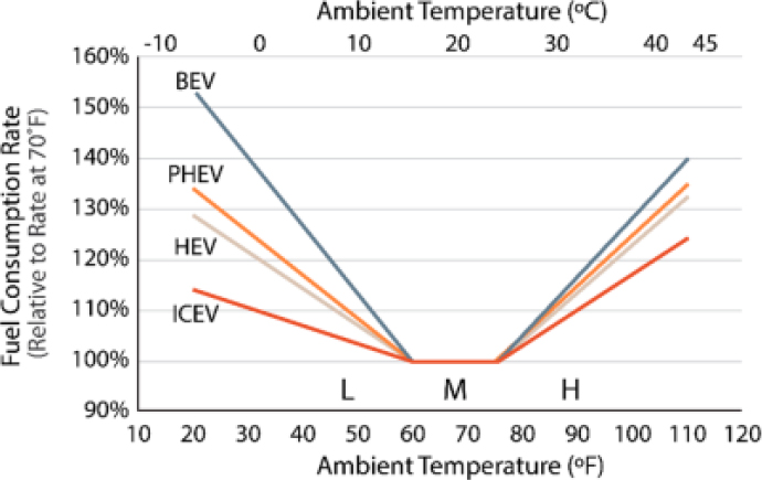
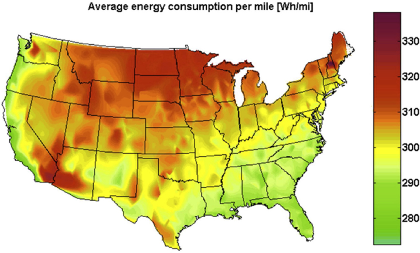
Simultaneous Variation in Vehicle Design and Multiple Use Conditions

When considering all of these factors together, using regional weather information, regional marginal emission factors, and regional differences in driving style (assuming city driving in urban counties, highway driving in rural counties, and combined driving in suburban counties), the comparison of life-cycle GHG emissions from gasoline and electric vehicles depends not only on which specific vehicle models are being compared but also on regional differences in climate, grid mix, and driving patterns (Yuksel et al., 2016).

While specific estimates of life-cycle GHG emissions for each vehicle type change over time and may vary across different LCA studies, depending on what assumptions are used and which vehicle models are used to represent each fuel type, the main point here is that there is so much variation across vehicle designs within each fuel type and across use conditions that using a single efficiency point estimate to represent each fuel type can substantially affect findings of an LCA, depending which vehicle design and use conditions are assumed. Use conditions, including driving style, climate, and energy source, all of which vary regionally, affect the emissions of vehicles for different fuel types differently and can affect which fuel type is estimated to have higher or lower life-cycle GHG emissions.

Fuel Octane Rating

Fuel octane ratings are standardized measurements of the ability of a fuel to withstand compression without detonation. Higher octane fuels can withstand higher compressions without premature combustion. Operating engines at higher compression can improve power and efficiency, although in modern engines this is just one variable of many.^8,9 Fuel properties affect internal combustion engine performance, and engine design and controls affect fuel needs. The combined effects of both result in measurable differences in performance, fuel consumption, and tailpipe emissions. Premature fuel combustion and engine knock were observed in gasoline internal combustion engines more than a hundred years ago, and various solutions have been implemented. Early solutions focused more on fuel composition, while more recent ones have focused on engine control, especially with the advent of controlling spark advance mechanically, and later electronically. This section discusses fuel octane rating as one key fuel specification with implications for fuel LCA. In order to ensure adequate octane ratings of finished fuels refiners add aromatic hydrocarbons (benzene, toluene, and xylene combined often referred to as BETX, plus others), which are molecules with high octane ratings. Ethanol, when blended into the fuel, has a high octane rating and therefore can dilute and substitute aromatics in gasoline. There has been a long history of using additives to increase octane rating by changing fuel composition. All of these have had positive impacts on engine performance but usually were found to have significant detrimental effects on health and the environment, which led to progressive banning of these additives. Most notoriously, the first additive in large-scale use, tetraethyl lead introduced in 1924, has been found to cause significant health damage, especially in children. It was removed gradually and finally banned in 1996. Methyl tertiary-butyl ether was introduced in the 1990s and was removed gradually over the next two decades due to ground water contamination issues and replaced with ethanol.¹⁰

Ethanol blending in gasoline increased rapidly between 1997 (0.31 percent) and 2016 (9.57 percent), driven by a combination of methyl tertiary-butyl ether replacement, Volumetric Ethanol Excise Tax Credit (VEETC) blending tax credits, the requirements of the RFS1 in 2005 and RFS2 in 2007, and changing economics of gasoline blending.¹¹ By 2016, almost all U.S. gasoline was blended with 10 percent ethanol.¹² The increased octane of ethanol allowed refiners to reduce the aromatic content of gasoline, which fell from 25 percent to 19 percent over the same time frame (EPA Fuel Trends Report 2017).

Fuels with high octane ratings allow vehicle manufacturers to increase the compression ratio in an engine, which enables that engine to extract more mechanical energy from a given mass of air–fuel mixture due to its higher thermal efficiency.¹³ This has attracted engine and emissions researchers to study and develop engines that utilize higher octane fuels (Costenoble and de Groot, 2020; DOE, 2017; Schifter et al., 2020; Storey et al., 2016; West et al., 2018; Yang et al., 2019). The reviewed studies show that optimized higher octane fuel engines may at least partially or more than fully compensate for ethanol’s lower volumetric fuel economy (due to its lower heating value) and result in increased energy economy ratio, which is defined as the energy consumption in British thermal unit (joule) of the conventional E10 vehicle divided by that of the alternative fuel (Unnasch and Browning, 2000). For example, Oak Ridge National Laboratory research finds that high-octane fuel can provide "an improvement in vehicle fuel efficiency in vehicles designed and dedicated to use the increased octane" (Theiss et al., 2016). Consequences including LUC implications may be assessed by CLCA. The findings related to high-octane fuel in this section describe the efficiency of the optimized fuel engine system rather than the broader issues associated with the lifecycle of ethanol, which are described at length in the rest of this report.

___________________

⁸ See https://www.eia.gov/energyexplained/gasoline/octane-in-depth.php.

⁹ See https://www.astm.org/d2700-21.html.

¹⁰ See https://archive.epa.gov/mtbe/web/html/faq.html.

¹¹ EPA fuel trends report, see https://nepis.epa.gov/Exe/ZyPDF.cgi?Dockey=P100T5J6.pdf.

¹² See EIA https://www.eia.gov/todayinenergy/detail.php?id=26092.

¹³ The compression ratio is defined as the ratio between the volume of the cylinder with the piston in the bottom position and in the top position. The higher this ratio, the greater will be the power output from a given engine.

Vehicle Production Emissions

For each transportation fuel, there are emissions associated with producing, maintaining, and managing the end of life of the vehicle that converts the fuel into transportation services. Emissions from producing and maintaining gasoline and ethanol vehicles are similar, but emissions from producing BEVs tend to be larger because of the large battery packs needed to store enough energy to deliver a vehicle range comparable to gasoline vehicles (Elgowainy et al., 2018; Karabasoglu and Michalek, 2013; Ma et al., 2012; Nealer and Hendrickson, 2015; Yuksel et al., 2016). This does not imply, however, that emissions from BEVs are higher on a per mile or per ton-mile basis, as emissions productions are allocated over the service life of vehicles in LCA. Estimates of the emissions from producing BEVs vary widely, and the technology is still in flux, with lithium ion chemistries varying in the amount of cobalt, nickel, magnesium, aluminum, iron, and other materials used, among other factors, including the type and origin of these metals and lithium (Deng et al., 2020; DOE, 2020; NASEM, 2021; Schmuch et al., 2018; Transportation Research Board and National Research Council, 2015).

Logistics

An additional issue, particularly relevant for LCA of electric trucks, is that some fuel types require powertrain designs that take up more space or weight, reducing the amount of cargo that can be transported. In particular, electric Class 8 trucks sized for long-distance range require large, heavy battery packs, reducing payload capacity, and requiring more truck trips to deliver the same quantity of goods (Figure 6-6; Sripad and Viswanathan, 2017). Use of a per-ton-mile functional unit can partially account for these differences when comparing transportation fuels, though logistical constraints can be complicated and nonlinear.

Different fuel types imply different logistical constraints and may impose changes on travel demand. In particular, BEVs substantially reduce payload for Class 8 trucks, and more truck travel is required to move the same amount of goods.

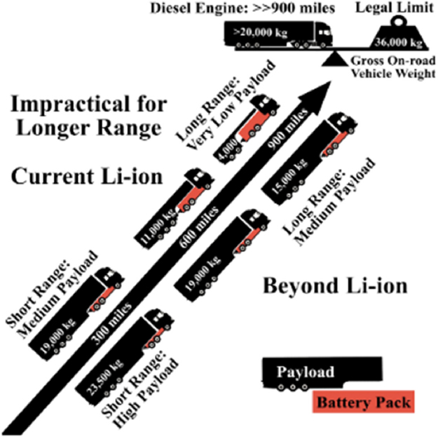
REFERENCES

Bernier, P. Y., R. L. Desjardins, Y. Karimi-Zindashty, D. Worth, A. Beaudoin, Y. Luo, and S. Wang. 2011. Boreal lichen woodlands: A possible negative feedback to climate change in eastern North America. Agricultural and Forest Meteorology 151(4):521–528.

Betts, R. A. 2000. Offset of the potential carbon sink from boreal forestation by decreases in surface albedo. Nature 408(6809):187–190.

Brandão, M., A. Levasseur, M. U. Kirschbaum, B. P. Weidema, A. L. Cowie, S. V. Jørgensen, M. Z. Hauschild, D. W. Pennington, and K. Chomkhamsri. 2013. Key issues and options in accounting for carbon sequestration and temporary storage in life cycle assessment and carbon footprinting. The International Journal of Life Cycle Assessment 18(1):230–240.

Brandão, M., M. U. F. Kirschbaum, A. L. Cowie, and S. V. Hjuler. 2019. Quantifying the climate change effects of bioenergy systems: Comparison of 15 impact assessment methods. GCB Bioenergy 11: 727–743. https://doi.org/10.1111/gcbb.12593.

Bredeson, L., R. Quiceno-Gonzalez, X. Riera-Palou, and A. Harrison. 2010. Factors driving refinery CO₂ intensity, with allocation into products. International Journal of Life Cycle Assessment 15:817–826. https://doi.org/10.1007/s11367-010-0204-3.

Buchholz, T., S. Prisley, G. Marland, C. Canham, and N. Sampson. 2014. Uncertainty in projecting GHG emissions from bioenergy. Nature Climate Change 4:1045–1047. https://doi.org/10.1038/nclimate2418.

Cai, H., J. Wang, Y. Feng, M. Wang, Z. Qin, and J. B. Dunn. 2016. Consideration of Land Use Change-Induced Surface Albedo Effects in Life-Cycle Analysis of Biofuels. Energy & Environmental Science 9(9):2855–67. https://doi.org/10.1039/C6EE01728B.

Cain, M., J. Lynch, M. R. Allen, J. S. Fuglestvedt, D. J. Frame, and A. H. Macey. 2019. Improved calculation of warming-equivalent emissions for short-lived climate pollutants. Climate and Atmospheric Science 2:29.

CARB. 2018. Carbon Capture and Sequestration Protocol under the Low Carbon Fuel Standard. 8/13/2018. https://ww2.arb.ca.gov/sites/default/files/2020-03/CCS_Protocol_Under_LCFS_8-13-18_ada.pdf.

CARB. 2020. Comment Log for Low Carbon Fuel Standard Public Workshop to Discuss Potential Regulation Revisions. https://www.arb.ca.gov/lispub/comm2/bccommlog.php?listname=lcfs-wkshp-oct20-ws.

CARB. 2021. LCFS Pathway Certified Carbon Intensities. https://ww2.arb.ca.gov/resources/documents/lcfs-pathway-certified-carbon-intensities.

Cherubini, E., D. Franco, G. M. Zanghelini, and S. R. Soares. 2018. Uncertainty in LCA case study due to allocation approaches and life cycle impact assessment methods. International Journal of Life Cycle Assessment 23:2055–2070. https://doi.org/10.1007/s11367-017-1432-6.

Cherubini, F., Bright, R.M. and Strømman, A.H., 2012. Site-specific global warming potentials of biogenic CO₂ for bioenergy: contributions from carbon fluxes and albedo dynamics. Environmental Research Letters 7(4), p.045902.

Cherubini, F., J. Fuglestvedt, T. Gasser, A. Reisinger, O. Cavalett, M. A. J. Huijbregts, D. J. A. Johansson, S. V. Jørgensen, A. Raugei, G. Schivley, A. H. Strømman, K. Tanaka, and A. Levasseur. 2016. Bridging the gap between impact assessment methods and climate science. Environmental Science & Policy 64:129–140.

Cherubini, F., G. P. Peter, T. Berntsen, A. H. Strømman, and E. Hertwich. 2011. CO₂ emissions from biomass combustion for bioenergy atmospheric decay and contribution to global warming. GCB Bioenergy 3(5):413–426.

Cintas, O., G. Berndes, A. L. Cowie, G. Egnell, H. Holmström, and G. I. Ågren. 2016. The climate effect of increased forest bioenergy use in Sweden: evaluation at different spatial and temporal scales. Wiley Interdisciplinary Reviews: Energy and Environment 5(3):351–369.

Collins, W.J., D. J. Frame, J. S. Fuglestvedt, and K. P. Shine. 2020. Stable climate metrics for emissions of short and long-lived species – combining steps and pulses. Environmental Research Letters 15:024018.

Colorado State University. n.d. DayCent: Daily Century Model. https://www2.nrel.colostate.edu/projects/daycent/ (accessed February 10, 2022).

Communication from the Commission on the practical implementation of the EU biofuels and bioliquids sustainability scheme and on counting rules for biofuels, 2010/C 160/02 § (n.d.).

Costenoble, O., and T. de Groot. 2020. Engine tests with new types of biofuels and development of biofuel standards. Report by the Netherlands Standardization Institute (NEN); Delft, The Netherlands. 2020-01-24. https://advancedbiofuelsusa.info/ortwin-costenoble-on-future-biofuels-standards-in-the-eu/.

Cowie, A. L., G. Berndes, N. S. Bentsen, M. Brandão, F. Cherubini, G. Egnell, B. George, L. Gustavsson, M. Hanewinkel, Z. M. Harris, and F. Johnsson. 2021. Applying a science‐based systems perspective to dispel misconceptions about climate effects of forest bioenergy. GCB Bioenergy 13(8):1210–1231. https://onlinelibrary.wiley.com/doi/epdf/10.1111/gcbb.12844.

Cowie, A., G. Berndes, and T. Smith. 2013. On the Timing of Greenhouse Gas Mitigation Benefits of Forest-Based Bioenergy (Vol. 4). IEA Bioenergy Executive Committee Statement. https://www.ieabioenergy.com/publications/on-the-timing-of-greenhouse-gas-mitigation-benefits-of-forest-based-bioenergy.

Darvin, E. L., S. I. Seneviratne, P. Ciais, A. Olioso, and T. Wang. 2014. Preferential cooling of hot extremes from cropland albedo management. Proceedings of the National Academies of Sciences of the United States of America 111(27):9757–9761.

De Kleine, R. D., T. J. Wallington, J. E. Anderson, and H. C. Kim. 2017. Commentary on “Carbon balance effects of US biofuel production and use” by DeCicco et al. (2016). Climatic Change 144:111–119. https://doi.org/10.1007/s10584-017-2032-y.

DeCicco, J. M. 2017. Author’s response to commentary on “Carbon balance effects of U.S. biofuel production and use.” Climatic Change 144:123–129. https://doi.org/10.1007/s10584-017-2026-9.

DeCicco, J.M., and W. H. Schlesinger. 2018. Reconsidering bioenergy given the urgency of climate protection. Proceedings of the National Academy of Sciences, 115(39), pp.9642-9645.

DeCicco, J. M., D. Y. Liu, J. Heo, R. Krishnan, A. Kurthen, and L. Wang. 2016. Carbon balance effects of US biofuel production and use. Climate Change 138:667–680.

Deng, J., C. Bae, A. Denlinger, and T. Miller. 2020. Electric vehicles batteries: requirements and challenges. Joule 4(3):511–515. https://www.sciencedirect.com/science/article/pii/S254243512030043X.

Denicoff, M. R., M. E. Prater, and P. Bahizi. 2014. Soybean Transportation Profile. USDA. https://www.ams.usda.gov/sites/default/files/media/Soybean%20Transportation%20Profile.pdf (accessed February 10, 2022).

Directive (EU). 2018. 2018/2001 of the European Parliament and of the Council of 11 December 2018 on the promotion of the use of energy from renewable sources, Pub. L. No. 32018L2001, OJ L 328 (2018). http://data.europa.eu/eli/dir/2018/2001/oj/eng.

DOE (US Department of Energy). 2017. U.S. Department of Energy, Office of Energy Efficiency and Renewable Energy, Vehicle Technologies Office. Advanced Combustion Systems and Fuels 2017 Annual Progress Report. https://www.energy.gov/sites/default/files/2018/05/f51/AdvCombSysAndFuels_FY2017_APR_Final.pdf (accessed February 11, 2022).

DOE. 2020. 2019 Annual Progress Report – Batteries. https://www.energy.gov/eere/vehicles/downloads/2019-annual-progress-report-batteries (accessed April 23, 2022).

Dwivedi, P., M. Khanna, A. Sharma, and A. Susaeta. 2016. Efficacy of Carbon and Bioenergy Markets in Mitigating Carbon Emissions on Reforested Lands: A Case Study from Southern United States. Forest Policy and Economics 67:1–9.

Dynarski, K., D. A. Bossio, and K. M. Scow. 2020. Dynamic Stability of Soil Carbon: Reassessing the “Permanence” of Soil Carbon Sequestration. Frontiers in Environmental Science 8. https://doi.org/10.3389/fenvs.2020.514701.

EIA (US Energy Information Administration). Gasoline Explained. Replaced by ASTM. https://www.eia.gov/energyexplained/gasoline/octane-in-depth.php (accessed February 10, 2022).

Elgowainy, A., J. Han, J. Ward, F. Joseck, D. Gohlke, A. Lindauer, T. Ramsden, M. Biddy, M. Alexander, S. Barnhart, and I. Sutherland. 2018. Current and future United States light-duty vehicle pathways: Cradle-to-grave lifecycle greenhouse gas emissions and economic assessment. Environmental Science & Technology 52(4):2392–2399.

Emery, I., S. Mueller, Z. Qin, and J. B. Dunn. 2017. Evaluating the potential of marginal land for cellulosic feedstock production and carbon sequestration in the United States. Environmental Science & Technology, 51(1):733–741. https://doi.org/10.1021/acs.est.6b04189.

EPA (Environmental Protection Agency). 2010. Renewable Fuel Standard Program (RFS2) Regulatory Impact Analysis. U.S. Environmental Protection Agency. EPA-420-R-10-006. https://19january2017snapshot.epa.gov/sites/production/files/2015-08/documents/420r10006.pdf.

EPA. 2014. Framework for Assessing Biogenic CO₂ Emissions from Stationary Sources, Office of Air and Radiation Office of Atmospheric Programs, Climate Change Division. United States Environmental Protection Agency, Washington DC. https://yosemite.epa.gov/Sab/Sabproduct.nsf/0/3235DAC747C16FE985257DA90053F252/$File/Framework-for-Assessing-Biogenic-CO2-Emissions+(Nov+2014).pdf).

EPA. 2017. Office of Transportation and Air Quality. Fuel Trends Report: Gasoline 2006 – 2016 EPA-420-R-17-005. https://nepis.epa.gov/Exe/ZyPDF.cgi?Dockey=P100T5J6.pdf (accessed February 10, 2022).

EPA. n.d. Methyl Tertiary Butyl Ether (MTBE). https://archive.epa.gov/mtbe/web/html/faq.html.

Ericsson, N., C. Porsö, S. Ahlgren, A. Nordberg, C. Sundberg, and P. A. Hansson. 2013. Time-dependent climate impact of a bioenergy system – methodology development and application to Swedish conditions. GCB Bioenergy 5(5):580–590.

European Commission. 2010. International Reference Life Cycle Data System (ILCD) Handbook – General guide for life cycle assessment – Detailed guidance. Joint Research Centre – Institute for Environment and Sustainability. EUR24708 EN, Publications Office of the European Union, Luxembourg.

Fargione, J., J. Hill, D. Tilman, S. Polasky, and P. Hawthorne. 2008. Land clearing and the biofuel carbon debt. Science 319(5867):1235–1238. https://www.science.org/doi/full/10.1126/science.1152747.

Field, J. L., H. Cai, M. S. Laser, D. S. LeBauer, S. P. Long, L. R. Lynd, K. Paustian, Z. Qin, T. L. Richard, J. J. Sheehan, P. Smith, E. A. H. Smithwick, and M. Q. Wang. 2020. Robust paths to net greenhouse gas mitigation and negative emissions via advanced biofuels. PNAS 117:21968–21977.

Forster, P., T. Storelvno, K. Armour, W. Collins, J. L. Dufresne, D. Frame, D. J. Lunt, T. Mauritsen, M. D. Palmer, M. Watanabe, M. Wild, and H. Zhang. 2021. The Earth’s Energy Budget, Climate Feedbacks, and Climate Sensitivity. In Climate Change 2021: The Physical Science Basis. Contribution of Working Group I to the Sixth Assessment Report of the Intergovernmental Panel on Climate Change. V. Masson-Delmotte, P. Zhai, A. Pirani, S. L. Connors, C. Péan, S. Berger, N. Caud, Y. Chen, L. Goldfarb, M. I. Gomis, M. Huang, K. Leitzell, E. Lonnoy, J. B. R. Matthews, T. K. May-cock, T. Waterfield, O. Yelekçi, R. Yu, B. Zhou, eds. Cambridge University Press.

Fuglestvedt, J., T. Berntsen, G. Myhre, K. Rypdal, and R. B. Skeie. 2008. Climate forcing from the transport sector. Proceedings of the National Academy of Sciences of the United States of America 105(2):454–458.

Giuntoli, J., S. Searle, R. Jonsson, A. Agostini, N. Robert, S. Amaducci, L. Marelli, and A. Camia. 2020. Carbon accounting of bioenergy and forest management nexus. A reality-check of modeling assumptions and expectations, Renewable and Sustainable Energy Reviews 134. https://doi.org/10.1016/j.rser.2020.110368.

GRAS (Global Risk Assessment). n.d. Sustainable, transparent & deforestation-free supply chains. https://www.gras-system.org/.

Haberl, H., D. Sprinz, B. Marc, P. Cocco, Y. Desaubies, M. Henze, O. Hertel, R. K. Johnson, U. Kastrup, P. Laconte, E. Lange, P. Novak, J. Paavola, A. Reenberg, S. van den Hove, T. Vermeire, P. Wadhams, and T. Searchinger. 2012. Correcting a fundamental error in greenhouse gas accounting related to bioenergy. Energy Policy 45:18–23.

Heijungs, R., K. Allacker, E. Benetto, M. Brandão, J. B. Guinee, S. Schaubroeck, T. Schaubroeck, and A. Zamagni. 2021. System expansion and substitution in LCA: A lost opportunity of ISO 14044 amendment 2. Frontiers in Sustainability 2.

Hicks Pries, C. E., C. Castanha, R. C. Porras, and M. S. Torn. 2017. The whole-soil carbon flux in response to warming. Science 355(6332):1420–1423. https://www.science.org/doi/abs/10.1126/science.aal1319. FN 21.

Holtsmark, B. 2015. A comparison of the global warming effects of wood fuels and fossil fuels taking albedo into account. Global Change Biology Bioenergy 7(5):984–997.

ICF International. 2015. Waste, Residue and By‐Product Definitions for the California Low Carbon Fuel Standard. Washington, DC: International Council on Clean Transportation, 2015. https://theicct.org/sites/default/files/publications/ICF_LCFS_Biofuel_Categorization_Final_Report_011816-1.pdf.

IPCC (Intergovernmental Panel on Climate Change). 1990. Climate Change: The IPCC Scientific Assessment. Contribution of Working Group I to the First Assessment Report of the Intergovernmental Panel on Climate Change. J.T. Houghton, G.H. Jenkins, J.J. Ephraums, eds. Cambridge University Press, United Kingdom, 365 p.

IPCC. 2019. Refinement to the 2006 IPCC Guidelines for National Greenhouse Gas Inventories (Vol 4). Agriculture, Forestry and Other Land Use. https://www.ipcc-nggip.iges.or.jp/public/2019rf/vol4.html (accessed February 10, 2022).

IPCC. n.d. Task Force on National Greenhouse Gas Inventories. http://www.ipcc-nggip.iges.or.jp/ (accessed February 10, 2022).

ISO (International Organization for Standardization). 2006. Environmental Management: Life Cycle Assessment; Requirements and Guidelines. ISO Geneva.

Jolliet, O., A. Antón, A. M. Boulay, F. Cherubini, P. Fantke, A. Levasseur, T. E. McKone, O. Michelsen, L. Milá i Canals, M. Motoshita, S. Pfister, F. Verones, B. Vigon, and R. Frischknecht. 2017. Global guidance on environmental life cycle impact assessment indicators: Impacts of climate change, fine particular matter formation, water consumption and land use. The International Journal of Life Cycle Assessment 23:2189–2207.

Jones, A. D., W. D. Collins, J. Edmonds, M. S. Torn, A. Janetos, K. V. Calvin, A. Thomson, L. P. Chini, J. F. Mao, X. Y. Shi, P. Thornton, G. C. Hurtt, and M. Wise. 2013. Greenhouse gas policy influences climate via direct effects of land-use change. Journal of Climate 26(11):3657–3670.

Jonker, J. G. G., M. Junginger, and A. Faaij. 2014. Carbon payback period and carbon offset parity point of wood pellet production in the South‐eastern United States. GCB Bioenergy 6(4):371–389. https://onlinelibrary.wiley.com/doi/full/10.1111/gcbb.12056.

Karabasoglu, O., and J. Michalek. 2013. Influence of driving patterns on life cycle cost and emissions of hybrid and plug-in electric vehicle powertrains. Energy Policy 60:445–461.

Kendall, A., B. Chang, and B. Sharpe. 2009. Accounting for time-dependent effects in biofuel life cycle greenhouse gas emissions calculations. Environmental Science & Technology 43:7142–7147.

Khanna, M., W. Wang, and M. Wang. 2020. Assessing the additional carbon savings with biofuel, BioEnergy Research 13:1082–1094. https://doi.org/10.1007/s12155-020-10149-0.

Lamers, P., and M. Junginger. 2013. The ‘debt’ is in the detail: A synthesis of recent temporal forest carbon analyses on woody biomass for energy. Biofuels, Bioproducts and Biorefining 7(4):373–385.

Lan, K., L. Ou, S. Park, S. S. Kelley, P. Nepal, H. Kwon, H. Cai, and Y. Yao. 2021. Dynamic life-cycle carbon analysis for fast pyrolysis biofuel produced from pine residues: implications of carbon temporal effects. Biotechnology Biofuels 14:191. https://doi.org/10.1186/s13068-021-02027-4.

Larrick, R. P., and J. B. Soll. 2008. The MPG illusion. Science 320(5883):1593–1594.

Ledo, A., J. Hillier, P. Smith, E. Aguilera, S. Blagodatskiy, F. Q. Brearley, A. Datta, E. Diaz-Pines, A. Don, M. Dondini, J. Dunn, D. M. Feliciano, M. A. Liebig, R. Lang, M. Llorente, Y. L. Zinn, N. McNamara, S. Ogle, Z. Qin, P. Rovira, R. Rowe, J. L. Vicente-Vicente, J. Whitaker, Q. Yue, and A. Zerihun. 2019. A global, empirical, harmonised dataset of soil organic carbon changes under perennial crops. Science Data 6:57. https://doi.org/10.1038/s41597-019-0062-1.

Leifeld, J., and S. G. Keel. 2022. Quantifying negative radiative forcing of non-permanent and permanent soil carbon sinks, Geoderma 423:115971.

Levasseur, A., O. Cavalett, J. S. Fuglestvedt, T. Gasser, D. J. A. Johansson, S. V. Jørgensen, M. Raugei, A. Reisinger, G. Schivley, A. Strømman, K. Tanaka, and F. Cherubini. 2016b. Enhancing life cycle impact assessment from climate science: Review of recent findings and recommendations for application to LCA. Ecological Indicators 71:163–174.

Levasseur, A., A. de Schryver, M. Hauschild, Y. Kabe, A. Sahnoune, K. Tanaka, and F. Cherubini. 2016a. Greenhouse gas emissions and climate change impacts. In R. Frischknecht, and O. Jolliet, eds. Global Guidance for Life Cycle Impact Assessment Indicators - Volume 1 (pp. 60–79): United Nations Environment Programme.

Levasseur, A., P. Lesage, M. Margni, M. Brandão, and R. Samson. 2012. Assessing temporary carbon sequestration and storage projects through land use, land-use change and forestry: Comparison of dynamic life cycle assessment with ton-year approaches. Climatic Change 115:759–776.

Levasseur, A., P. Lesage, M. Margni, L. Deschênes, and R. Samson. 2010. Considering time in LCA: Dynamic LCA and its application to global warming impact assessments. Environmental Science & Technology 44:3169–3174.

Ma, H., F. Balthasar, N. Tait, X. Riera-Palou, and A. Harrison. 2012. A new comparison between the life cycle greenhouse gas emissions of battery electric vehicles and internal combustion vehicles. Energy policy 44:160–173. https://www.sciencedirect.com/science/article/abs/pii/S0301421512000602#f0025.

McKechnie, J., S. Colombo, J. Chen, W. Mabee, and H. L. MacLean. 2011. Forest bioenergy or forest carbon? Assessing trade-offs in greenhouse gas mitigation with wood-based fuels. Environmental Science & Technology 45(2):789–795.

Mueller, S., G. Dennison, and S. Liu. 2021. An assessment on ethanol-blended gasoline/diesel fuels on cancer risk and mortality. International Journal of Environmental Research 18:6930. Public Health. https://doi.org/10.3390/ijerph18136930.

Muñoz, I., P. Campra, and A. R. Fernández-Alba. 2010. Including CO₂-emission equivalence of changes in land surface albedo in life cycle assessment. Methodology and case study on greenhouse agriculture. The International Journal of Life Cycle Assessment 15:672–681.

Myhre, G., D. Shindell, F. M. Bréon, W. Collins, J. Fuglestvedt, J. Huang, D. Koch, J. F. Lamarque, D. Lee, B. Mendoza, T. Nakajima, A. Robock, G. Stephens, T. Takemura, and H. Zhang. 2013. Anthropogenic and Natural Radiative Forcing. In T.F Stocker, D. Qin, G.K. Plattner, M. Tignor, S.K. Allen, J. Boschung, A. Nauels, Y. Xia, V. Bex, and P.M. Midgley, eds. Climate Change 2013: The Physical Science Basis. Contribution of Working Group I to the Fifth Assessment Report of the Intergovernmental Panel on Climate Change. Cambridge University Press, Cambridge, United Kingdom and New York, NY.

NASEM (National Academies of Sciences, Engineering, and Medicine). 2019. Negative Emissions Technologies and Reliable Sequestration: A Research Agenda. Washington, DC: The National Academies Press. https://doi.org/10.17226/25259.

NASEM. 2021. Assessment of Technologies for Improving Light-Duty Vehicle Fuel Economy—2025-2035. Washington, DC: The National Academies Press. https://doi.org/10.17226/26092.

Nealer, R., and T. P. Hendrickson. 2015. Review of recent lifecycle assessments of energy and greenhouse gas emissions for electric vehicles. Current Sustainable/Renewable Energy Reports 2:66–73. https://doi.org/10.1007/s40518-015-0033-x.

O’Hare, M., R. J. Plevin, J. I. Martin, A. D. Jones, A. Kendall, and E. Hopson. 2009. Proper accounting for time increases crop-based biofuels’ greenhouse gas deficit versus petroleum. Environmental Research Letters 4:024001.

Parton, W. J. 1996. The CENTURY model. In D.S. Powlson, P. Smith, J.U. Smith. eds. Evaluation of Soil Organic Matter Models. NATO ASI Series (Series I: Global Environmental Change), Vol 38. Springer, Berlin, Heidelberg. https://doi.org/10.1007/978-3-642-61094-3_23.

Peñaloza, D., F. Røyne, G. Sandin, M. Svanström, and M. Erlandsson. 2019. The influence of system boundaries and baseline in climate impact assessment of forest products. International Journal of Life Cycle Assessment 24:160–176. https://doi.org/10.1007/s11367-018-1495-z.

Qin, Z., J. B. Dunn, H. Kwon, S. Mueller, and M. M. Wander. 2014. Soil carbon sequestration and land use change associated with biofuel production: Empirical evidence. GCB Bioenergy 8:66–80. https://doi.org/10.1111/gcbb.12237.

Red Trail Energy. 2019. Red Trail Energy Low Carbon Fuel Standard (LCFS) Design-Based Pathway Application – Carbon Capture and Storage Integrated with Ethanol Production. Red Trail Energy. Richardton, ND.

Schifter, I., L. Díaz, G. Sánchez-Reyna, C. González-Macías, U. González, and R. Rodríguez. 2020. Influence of gasoline olefin and aromatic content on exhaust emissions of 15% ethanol blends. Fuel 265:116950.

Schmuch, R., R. Wagner, G. Hörpel, T. Placke, and M. Winter. 2018. Performance and cost of materials for lithium-based rechargeable automotive batteries. Nature Energy 3:267–278. https://doi.org/10.1038/s41560-018-0107-2.

Schrijvers, D. L., P. Loubet, and G. Sonnemann. 2016. Developing a systematic framework for consistent allocation in LCA. International Journal of Life Cycle Assessment 21:976–993. https://doi.org/10.1007/s11367-016-1063-3.

Searchinger, T. D. 2010. Biofuels and the need for additional carbon. Environmental Research Letters 5:24007.

Searchinger, T., S. P. Hamburg, J. Melillo, W. Chameides, P. Havlik, D. M. Kammen, G. E. Likens, R. N. Lubowski, M. Obersteiner, M. Oppenheimer, G. P. Robertson, W. H. Schlesinger, and G. D. Tilman. 2009. Fixing a critical climate accounting error. Science 326:527–528.

Searchinger, T., R. Heimlich, R. A. Houghton, F. Dong, A. Elobeid, J. Fabiosa, S. Tokgoz, D. Hayes, and T. H. Yu. 2008. Use of US croplands for biofuels increases greenhouse gases through emissions from land-use change. Science 319(5867):1238–1240. https://www.science.org/doi/10.1126/science.1151861.

Sieber, P., N. Ericsson, T. Hammar, and P. A. Hansson. 2020. Including albedo in time-dependent LCA of bioenergy. GCB Bioenergy 12(6):410–425.

Sieber, P., N. Ericsson, and P.A. Hansson. 2019. Climate impact of surface albedo change in life cycle assessment: Implications of site and time dependence. Environmental Impact Assessment Review 77:191–200.

Seber, G., R. Malina, M. N. Pearlson, H. Olcay, J. I. Hileman, and S. R. Barrett. 2014. Environmental and economic assessment of producing hydroprocessed jet and diesel fuel from waste oils and tallow. Biomass and Bioenergy 67:108–118.

Shine, K. P. P., R. P. P. Allan, W. J. J. Collins, and J. S. S. Fuglestvedt. 2015. Metrics for linking emissions of gases and aerosols to global precipitation changes. Earth System Dynamics 6(2):525–540.

Shine, K., J. Flugestvedt, K. Hailemariam, and N. Stuber. 2005. Alternatives to the global warming potential for comparing climate impacts of emissions of greenhouse gases. Climatic Change 68:281–302.

Smith, M. A., M. Cain, and M. R. Allen. 2021. Further improvement of warming-equivalent emissions calculation. Climate and Atmospheric Science 4:19.

Sripad, S., and V. Viswanathan. 2017. Performance metrics required of next generation batteries to make a practical electric semi-truck. ACS Energy Letters 2:1669−1673. https://pubs.acs.org/doi/pdf/10.1021/acsenergylett.7b00432 (accessed February 10, 2022).

Storey, J., M. DeBusk, S. Huff, S. Lewis, F. Li, J. Thomas, and M. Eibl. 2016. Characterization of GDI PM during start-stop operation with alcohol fuel blends. Oak Ridge National Laboratory. Presented at Effects of Fuel Composition on PM Health Effects Institute Workshop, December 8, 2016. Chicago, IL. https://www.healtheffects.org/sites/default/files/Storey-Characterization_of_GDI_PM.pdf. (accessed February 11, 2022).

Theiss, T. J., T. Alleman, A. Brooker, A. Elgowainy, G. Fioroni, Gina, J. Han, Jeongwoo, S. P. Huff, C. Johnson, M. D. Kass, P. N. Leiby, R. U. Martinez, R. McCormick, K. Moriarty, E. Newes, G. A. Oladosu, J. P. Szybist, J. F. Thomas, M. Wang, and B. H. West. 2016. Summary of High-Octane Mid-Level Ethanol Blends Study. ORNL/TM-2016/42, 1286966. Oak Ridge National Laboratory. https://doi.org/10.2172/1286966.

Tillman, A.-M. 2000. Significance of decision-making for LCA methodology. Environmental Impact Assessment Review 20(1):113–123. https://doi.org/10.1016/S0195-9255(99)00035-9.

Transportation Research Board and National Research Council. 2015. Overcoming Barriers to Deployment of Plug-in Electric Vehicles. The National Academies Press, Washington, DC. https://doi.org/10.17226/21725.

U.K. Department for Transport. Renewable Transport Fuel Obligation Guidance Part Two Carbon and Sustainability. London, UK: UK Department for Transport. 2021. https://assets.publishing.service.gov.uk/government/uploads/system/uploads/attachment_data/file/947710/rtfo-guidance-part-2-carbon-and-sustainability-2021.pdf.

U.K. Department for Transport. RTFO Guidance Year 10: Carbon & Sustainability Guidance. London, U.K.: U.K. Department for Transport. 2018. https://assets.publishing.service.gov.uk/government/uploads/system/uploads/attachment_data/file/604627/rtfo-guidance-part-2-carbon-sustainability-guidance-year-10.pdf.

USDA (US Department of Agriculture). 2020. Agricultural Marketing Service; 7 CFR Part 205. https://www.govinfo.gov/content/pkg/FR-2020-08-05/pdf/2020-14581.pdf.

Unnasch, S., and L. Browning. 2000. Fuel Cycle Energy Conversion Efficiency Analysis. California Energy Commission and Air Resources Board, California, viewed, 11, 07-12 with follow in analysis in Unnasch, S. and Chan, M. (2007) Full Fuel Cycle Assessment Tank to Wheels Emissions and Energy Consumption. California Energy Commission Report CEC-600-2007-003-D.

Verity Tracking. 2022. Measurement, Reporting, Verification and Value. https://www.veritytracking.com/.

Wang, M., J. Kelly, H. Kwon, X. Liu, Z. Lu, L. Ou, P. Sun, O. Winjobi, H. Xu, E. Yoo, G. Zaimes, and G. Zang. 2020. Greenhouse Gases, Regulated Emissions, and Energy Use in Technologies Model ® (2020 Excel). Argonne National Laboratory (ANL), Argonne, IL, United States. https://doi.org/10.11578/GREET-EXCEL-2020/DC.20200912.1.

Wang, M., J. Han, J. B. Dunn, H. Cai, and A. Elgowainy. 2012. Well-to-wheels energy use and greenhouse gas emissions of ethanol from corn, sugarcane and cellulosic biomass for US use. Environmental Research Letters, 7:045905.

Wang, M., H. Hong, and S. Arora. 2011. Methods of dealing with co-products of biofuels in life-cycle analysis and consequent results within the U.S. context. Energy Policy 39(10):5726–36. https://doi.org/10.1016/j.enpol.2010.03.052.

Weidema, B. 1999. System Expansions to Handle Co-Products of Renewable Materials 4, 45–48 in Presentation Summaries of the 7th LCA Case Studies Symposium SETAC-Europe. https://lca-net.com/files/casestudy99.pdf (accessed February 10, 2022).

West, B., S. Huff, L. Moore, M. DeBusk, and S. Sluder. 2018. Effects of High-Octane E25 on Two Vehicles Equipped with Turbocharged, Direct-Injection Engines. ORNL/TM-2018/814; September 2018. https://info.ornl.gov/sites/publications/Files/Pub109556.pdf (accessed February 10, 2022).

Wiloso, E. I., R. Heijungs, G. Huppes, and K. Fang. 2016. Effect of biogenic carbon inventory on the life cycle assessment of bioenergy: Challenges to the neutrality assumption. Journal of Cleaner Production 125:78–85. https://www.sciencedirect.com/science/article/pii/S0959652616301676#bib21.

Wu, D., F. Guo, F. R. Field III, R. D. De Kleine, H. C. Kim, T. J. Wallington, and R. E. Kirchain. 2019. Regional heterogeneity in the emissions benefits of electrified and lightweighted light-duty vehicles. Environmental Science & Technology 53(18):10560–10570. https://pubs.acs.org/doi/10.1021/acs.est.9b00648.

Xu, H., H. Sieverding, H. Kwon, D. Clay, C. Stewart, J. M. Johnson, Z. Qin, D. L. Karlen, and M. Wang. 2019. A global meta‐analysis of soil organic carbon response to corn stover removal. GCB Bioenergy 11(10):1215–1233. https://doi.org/10.1111/gcbb.12631.

Yang, J., P. Roth, T. D. Durbin, M. M. Shafer, J. Hemming, D. S. Antkiewicz, A. Asa-Awuku, and G. Karavalakis. 2019. Emissions from a flex fuel GDI vehicle operating on ethanol fuels show marked contrasts in chemical, physical and toxicological characteristics as a function of ethanol content. Science of the Total Environment 683:749–761. https://www.energy.gov/sites/default/files/2018/05/f51/AdvCombSysAndFuels_FY2017_APR_Final.pdf.

Yuksel, T., and J. J. Michalek. 2015. Effects of regional temperature on electric vehicle efficiency, range, and emissions in the United States. Environmental Science & Technology 49(6):3974–3980.

Yuksel, T., M. Tamayao, C. Hendrickson, I. Azevedo, and J. J. Michalek. 2016. Effect of regional grid mix, driving patterns and climate on the comparative carbon footprint of electric and gasoline vehicles. Environmental Research Letters 11(4):044007.

Zanchi, G., N. Pena, and N. Bird. 2012. Is woody bioenergy carbon neutral? A comparative assessment of emissions from consumption of woody bioenergy and fossil fuel. GCB Bioenergy 4(6):761–772.

Zhang, Y., J. M. Lavallee, A. D. Robertson, R. Even, S. M. Ogle, K. Paustian, and M. F. Cotrufo. 2021. Simulating measurable ecosystem carbon and nitrogen dynamics with the mechanistically defined MEMS 2.0 model, Biogeosciences 18:3147–3171. https://doi.org/10.5194/bg-18-3147-2021.

REFERENCES

Allen, R. J., S. Turnock, P. Nabat, D. Neubauer, U. Lohmann, D. Olivié, N. Oshima, M. Michou, T. Wu, J. Zhang, T. Takemura, M. Schulz, K. Tsigaridis, S. E. Bauer, L. Emmons, L. Horowitz, V. Naik, T. v. Noije, T. Bergman, J.-F. Lamarque, P. Zanis, I. Tegen, D. M. Westervelt, P. Le Sager, P. Good, S. Shim, F. O’Connor, D. Akritidis, A. K. Georgoulias, M. Deushi, L. T. Sentman, J. G. John, S. Fujimori, and W. J. Collins. 2020. Climate and air quality impacts due to mitigation of non-methane near-term climate forcers. Atmospheric Chemistry and Physics 20:9641–9663.
ASTM (American Society for Testing and Materials). 2021. Standard Test Method for Motor Octane Number of Spark-Ignition Engine Fuel. https://www.astm.org/d2700-21.html (accessed March 10, 2022).
Berndes, G., S. Ahlgren, P. Börjesson, and A. Cowie. 2013. Bioenergy and land use change—state of the art. WIREs Energy and Environment 2:282–303.