
4
Key Considerations: Direct and Indirect Effects, Uncertainty, Variability, and Scale of Production
This chapter addresses key considerations for applying life-cycle assessment (LCA) methods to transportation fuels, including three topics: (1) the definitions of direct and indirect effects, including supply chain and market-mediated effects triggered by fuel production and use, (2) characterization of uncertainty, and (3) issues with predicting emissions as a function of the scale of fuel production. The committee’s conclusions and recommendations on each of the topics are included in their respective sections.
DIRECT AND INDIRECT EFFECTS
Definitions of Direct and Indirect Effects in the Life-Cycle Assessment Context
One of the challenges in discussing the use of LCA in a proposed national low-carbon fuel standard (LCFS) is the inconsistent use of terminology. The guidelines in the International Organization for Standardization (ISO) 14040/14044 (ISO, 2006 2006a,b) provide a common language with which to discuss many aspects of the basic process of conducting an LCA, but they do not define the terms “direct” or “indirect.” The terms direct and indirect effects (or emissions) have been frequently used in LCA textbooks, regulatory documents, standards, and studies; however, definitions vary. Hertwich and Wood (2018) note that “different expert communities have developed a bewildering diversity of terms for indirect emissions… which is both a testimony to their importance and an opportunity for a more consistent terminology to ease communication.”
Broadly speaking, direct emissions are defined in various references as those emissions released from focal activities, sources or processes, and indirect emissions are those emissions released from non-focal activities, sources, or processes triggered by or induced by the focal activities (Argonne National Laboratory, n.d.-b; Carnegie Mellon University, n.d.; Hertwich and Wood, 2018; Matthews et al., 2014). Here the term “focal” is used to refer to whatever activities are the focus of the study, which differ across study contexts.
Table 4-1 summarizes how various references including regulatory documents, standards, textbooks, and studies define direct and indirect effects. For example, in some definitions the focal activities are those owned or controlled by a focal entity: direct emissions are those emissions released from sources owned or controlled by the focal entity, and indirect emissions are those from sources not owned or controlled by the focal entity but related to its activities (U. S. Environmental Protection Agency [EPA], Greenhouse Gas (GHG) Protocol, Economic Input–Output LCA, Hertwich and Wood [2018]). This definition of activities is often used by companies or government entities who wish to distinguish between emissions they control and emissions triggered by their activities or purchases but released by entities that they do not control. In other definitions, focal activities are those associated with a particular process, a supply chain, or an economic sector.
LCA studies differ substantially in how they choose focal activities and define direct and indirect emissions. For example, an analysis may center on a single facility, and all emissions that occur at the facility itself are considered direct, while all off-site emissions sources (e.g., grid-connected power plants supplying electricity) are indirect. Other analyses may consider all major activities within a fuel’s supply chain to be from focal activities (e.g., farming, transportation, biorefining, fuel combustion) and will call any emissions from those activities direct emissions while calling “upstream” supply chain sources, such as fertilizer manufacturing, indirect. Some studies use the term “indirect” to refer to market-mediated effects, such as indirect land use change (ILUC).
TABLE 4-1 Definitions of Direct and Indirect Emissions in the Literature
| Source | Definition |
|---|---|
| Carnegie Mellon University (n.d.): Economic Input Output Life Cycle Assessment |
Economic sector and first-tier suppliers “in all cases the environmental results are the total impacts, directly from the sector of interest and its direct (first-tier) suppliers and indirectly from all other sector transactions further up the supply chain.” |
| EPA (2021) |
Entity “Scope 1 GHG emissions are direct emissions from sources that are owned or controlled by the Agency. Scope 1 includes on-site fossil fuel combustion and fleet fuel consumption. Scope 2 GHG emissions are indirect emissions from sources that are owned or controlled by the Agency. Scope 2 includes emissions that result from the generation of electricity, heat or steam purchased by the Agency from a utility provider. Scope 3 GHG emissions are from sources not owned or directly controlled by EPA but related to Agency activities. Scope 3 emissions include employee travel and commuting. Scope 3 also includes emissions associated with contracted solid waste disposal and wastewater treatment. Some Scope 3 emissions can also result from transportation and distribution (T&D) losses associated with purchased electricity.” |
| EPA (2016) |
Entity “Indirect emissions are those that result from an organization’s activities, but are actually emitted from sources owned by other entities.” |
| GHG Protocol |
Entity “Direct GHG emissions are emissions from sources that are owned or controlled by the reporting entity. Indirect GHG emissions are emissions that are a consequence of the activities of the reporting entity, but occur at sources owned or controlled by another entity. The GHG Protocol further categorizes these direct and indirect emissions into three broad scopes: Scope 1: All direct GHG emissions. Scope 2: Indirect GHG emissions from consumption of purchased electricity, heat or steam. Scope 3: Other indirect emissions, such as the extraction and production of purchased materials and fuels, transport-related activities in vehicles not owned or controlled by the reporting entity, electricity-related activities (e.g. T&D losses) not covered in Scope 2, outsourced activities, waste disposal, etc.” |
| GREET CCLUB (2016) |
Domestic vs. international land use “The Carbon Calculator for Land Use Change from Biofuels Production (CCLUB) module was released by Argonne as an Excel spreadsheet that functions both as a standalone model and as a component of GREET. CCLUB estimates the direct (domestic) and indirect (international) emissions that occur as a result of land use changes during the production of ethanol.” |
| Hertwich and Wood (2018) |
Activities Direct emissions: Emissions directly associated with an activity, a process, or an entity Indirect emissions: Emissions associated with the production of the inputs to an activity or organization |
| ISO 14040 Series (LCA) | Not defined |
| Lave, Hendrickson and McMichael (1995) |
Economic sector “The direct economic changes associated with a choice are forecast. For example, switching from steel to aluminum for many automobile components would be represented by an increase in aluminum demand and a decrease in steel demand. An economic input-output model then is used to estimate both direct and indirect changes in output throughout the economy for each sector.” |
| Matthews et al. (2014) |
Activities “LCA models are able to capture direct and indirect effects of systems. In general, direct effects are those that happen directly as a result of activities in the process in question. Indirect effects are those that happen as a result of the activities, but outside of the process in question. For example, steel making requires iron ore and oxygen directly, but also electricity, environmental consulting, natural gas exploration, production, and pipelines, real estate services, and lawyers. Directly or indirectly, making cars involves the entire economy, and getting specific mass and energy flows for the entire economy is impossible.” |
A few concrete examples from the literature include (emphasis on terms “direct” and “indirect” added):
- In Searchinger et al. (2008): “To produce biofuels, farmers can directly plow up more forest or grass-land, which releases to the atmosphere … carbon … Alternatively, farmers can divert existing crops or croplands into biofuels, which causes … emissions indirectly.”
- In Bento and Klotz (2014) the delineation between direct and indirect “is based on the application and context being studied and determines the allocation procedures used to assign emissions to a technology, data choice, and the treatment of market-induced, or indirect, adjustments.... For evaluating changes, consequential LCA offers distinct advantages over the attributional approach, particularly in recognizing that market adjustments and indirect effects can be as important as the physical flows captured by attributional LCA, with indirect land use change (LUC) resulting from expanded biofuel production being a key example.”
- In Pehl et al. (2017): Direct emissions include direct fossil CO2 (with imperfect carbon capture). Indirect emissions include land use change (LUC), upstream and biogeneic CH4 operation, construction, bioenergy with carbon capture and storage.
- In Hertel et al. (2010) emissions from land use changes are indirect as noted by these authors: “…greenhouse gas (GHG) releases from indirect (or induced) land-use change (ILUC) triggered by crop-based biofuels…” On the other hand, according to these authors emissions from producing feedstock and conversion to biofuel is direct: “Direct releases of GHG also occur during the cultivation and industrial processing of maize ethanol. Estimates of these, not including ILUC.”
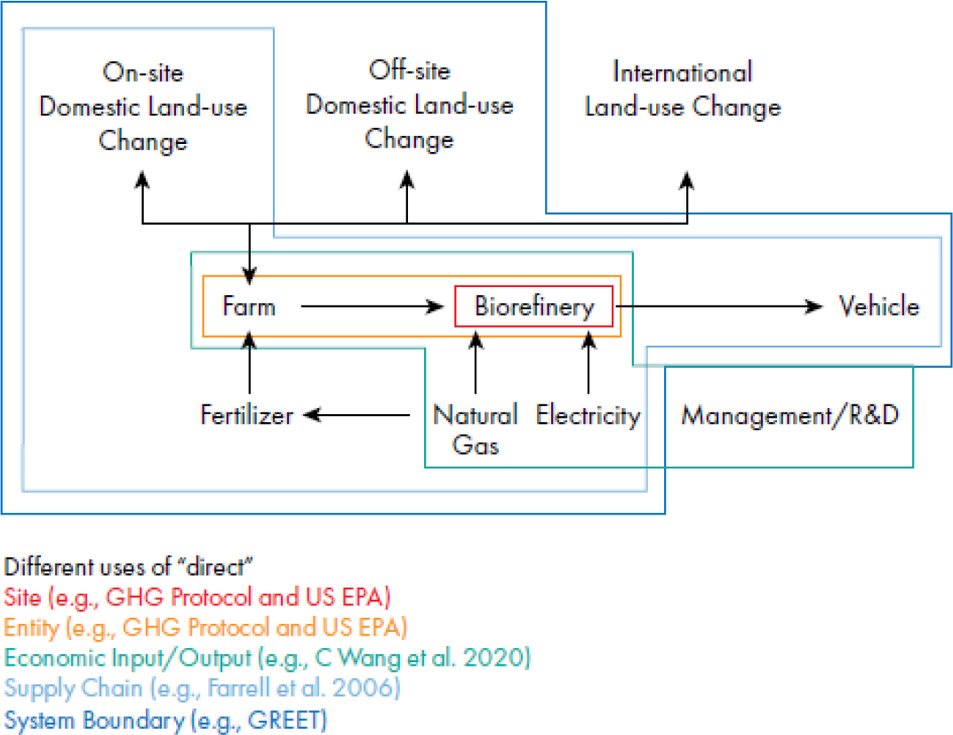
Figure 4-1 provides examples of how the boundaries between direct and indirect emissions differ across a selection of corn ethanol LCA studies and standards. Note that this figure shows the delineation between what is considered direct versus indirect in each study, not necessarily the system boundary (see Chapter 3).
Despite all of this variation, across all alternative sources that the committee reviewed, some emissions sources are almost universally considered to be direct (e.g., on-site emissions from a biorefinery in a corn ethanol LCA) and some emissions sources are almost universally considered to be indirect (e.g., emissions resulting from induced international LUCs due to market-mediated responses).
Understanding “Direct” and “Indirect” in Attributional and Consequential Life-Cycle Assessment
The concepts of direct and indirect emissions are distinct from the concepts of attributional and consequential emissions, but in some studies these ideas are conflated. For example, the GHG Protocol states “Indirect GHG emissions are emissions that are a consequence of the activities of the reporting entity.” Some LCA studies of biofuels estimate fuel supply chain emissions using attributional LCA (ALCA) and refer to these as “direct emissions” but add consequential estimates of induced LUC as “indirect emissions.” Table 4-2 shows the relationship between these concepts. Because some studies use ALCA to model “direct” emissions from focal activities (top left) and use consequential LCA (CLCA) to model “indirect” emissions from non-focal activities (bottom right), the terms can sometimes become conflated in the literature.
TABLE 4-2 Relationship between Direct/Indirect Emissions and Attributional/Consequential LCA
| Attributional | Consequential | |
|---|---|---|
| Direct | Assigned (e.g., average) emissions from focal processes or activities | Change in emissions from focal sources due to an action or decision |
| Indirect | Assigned (e.g., average) emissions from other sources induced by the focal processes or activities | Change in emissions from other sources due to an action or decision |
Table 4-3 provides some examples of factors that may be considered direct or indirect effects associated with expansions in biofuels and electric vehicles (EVs). These categorizations vary across studies and sources, and this table does not provide a definitive list of which effects should be referred to as direct or indirect: rather, Table 4-3 offers concrete examples of these types of effects. The terms “direct” and “indirect” are used frequently in biofuels LCA studies (see Chapter 9), but they are not used commonly in EV LCA studies (see Chapter 10). This may be, in part, because many biofuels studies use ALCA to model the partial supply chain but include induced LUC as an added consequential element outside the ALCA boundary ever since the issue was raised as a critical factor by Searchinger et al. (2008). In contrast, most modern EV LCA studies model power sector emissions using CLCA, estimating how power grid emissions will change in response to changes in EV charging load (see Chapter 10 for a list of studies) but do not necessarily model other market-mediated effects, such as rebound. Because CLCA is typically not focused on assigning emissions to products or activities, the distinction between direct and indirect has not been useful terminology to adopt in most of the EV LCA literature. However, we provide examples in Table 4-3 to emphasize that both biofuels and EVs (as well as other fuels) have market-mediated effects.
| Direct/Indirect | Biofuel Examples | Electric Vehicle Examples |
|---|---|---|
| Potentially referred to as direct effects | Emissions from corn and soybeans in supply chain of an ethanol or biodiesel plant (Plevin et al., 2014a) | N/A |
| Potentially referred to as indirect effects |
Land use emissions and sequestration effects due to changes in demand for a given feedstock:
|
Induced emissions due to changes in demand for electricity:
|
| Potentially referred to as indirect effects due to rebound or fuel market price effects |
|
|
| Direct/Indirect | Biofuel Examples | Electric Vehicle Examples |
|---|---|---|
|
|
|
Finally, it should be noted that calling effects “direct” or “indirect” has no bearing on their relative contribution to overall life-cycle impacts. Major sources of emissions can include those within and beyond the focal activities (Matthews et al., 2008; Meinrenken and Lackner, 2015; Meinrenken et al., 2020).
In sum, the terms “direct” and “indirect” are defined and used differently in different regulatory documents, standards, practices, scientific references, and LCA methods, and there are no universally accepted definitions. It is again worth noting that the ISO 14040 series standard for LCA does not use the terms “direct” or “indirect” in relation to effects or emissions.
The distinction between direct and indirect emissions is commonly based on what a given study identifies as focal activities. These are typically based on the source of emissions, the entities that generate the emissions, or, in the case of some approaches that mix ALCA and CLCA, the ALCA system boundary used in the analysis.
Some ALCA studies use the ALCA system boundary to define focal activities but also add other factors beyond the ALCA system boundary, such as CLCA estimates of induced land use change due to market-mediated responses, and label all activities captured by the ALCA system boundary as direct effects. These studies label all activities outside the ALCA system boundary as indirect.
Conclusion 4-1: Dividing emissions into direct and indirect can be used when identifying and classifying sources of emissions, but it can cause confusion, even if carefully defined and transparently presented in an LCA.
Conclusion 4-2: Direct and indirect emissions are concepts distinct from the concepts of attributional and consequential LCA.
Recommendation 4-1: Because the terms “direct” and “indirect” are used differently in different contexts, these terms should be carefully defined and transparently presented when used in LCA studies or policy. Another option is to avoid using the terms “direct” and “indirect” altogether, as they are not considered necessary elements of LCA and may lead to greater confusion.
UNCERTAINTY AND VARIABILITY
LCAs are subject to considerable uncertainty and variability, and LCA methods need to appropriately characterize uncertainty and variability to aid LCA stakeholders’ interpretation of LCA results. The appropriate tool for uncertainty and variability analysis depends on the nature of the uncertainty and variability as well as the decisions or policies the LCA is intended to support. Accordingly, this section begins with general background on the types of uncertainty and variability and the methods that are used for uncertainty and variability characterization. It then proceeds to discuss specific uncertainties and variabilities in the context of low-carbon transportation fuels. Finally, it addresses the types of outputs that LCAs need to produce so that policymakers can be appropriately informed as to the range of possible outcomes.
Types of Uncertainty and Methods for Analysis
Uncertainty refers to a lack of knowledge. Variability refers to any difference in outcomes of different trials of a process. The differences may be understood and predictable based on underlying differences in the conditions under which the trials take place. An example of this would be known variation in electric power sources across different regions. In other cases, the variation may be due to inherent randomness of outcomes, generally termed aleatory factors, for example, a roll of the dice. Whether variability contributes to uncertainty depends on context, that is how much of the variation is inherent versus explained by known factors, and whether the explanatory factors are known. Uncertainty can come both from such aleatory factors and also from uncertainty in knowledge of the system in question, generally termed epistemic uncertainty. An example of epistemic uncertainty is the location of Genghis Khan’s tomb. There is no variability present as the tomb is located in one specific place, but that location is unknown. Such epistemic uncertainty may be reducible by further research and data collection. Both aleatory and epistemic uncertainty can be present in input parameters and data used in mathematical models.
Different definitions of uncertainty are described in the literature. ISO standard 14040 mentions model imprecision, input uncertainty, and data variability (ISO, 2006a). For LCA, examples of model input uncertainty include data related to process inputs, as well as environmental emissions and technology characteristics, most of which are associated with life-cycle inventory (LCI) data (Lloyd and Ries, 2007). Precision can be understood to refer to variability, such as observations’ deviation from their collective mean. Furthermore, ISO 14044 discusses the use of uncertainty analysis to determine the effects of uncertainties in empirical quantities and in modeling assumptions (ISO, 2006b). However, ISO standards do not provide detailed methodological guidance on uncertainty analysis. For example, the weather may influence the yield and ultimately the carbon intensity (CI) of biofuel feedstock cultivation, but the specific weather years in the future is inherently unpredictable. Both aleatory and epistemic uncertainty can be present in input parameters and data used in mathematical models.
Uncertainty is also generally present in the scenarios that analysts should consider. Scenarios consist of coherent sets of model inputs and parameters that reflect conditions of interest such as the times and locations at which activities will take place. They may also include the policy regime or broader market conditions that will apply to the analysis. Examples include common LCA modeling decisions such as choosing a functional unit, allocation methods, end-of-life scenarios, time frame, and geographic scales.
The fundamental assumptions underlying the structure of an analysis represent another form of uncertainty (Lloyd and Ries, 2007; Morgan and Henrion, 1990). In LCA a common example of this is the uncertainty in the structure and mathematical relationships of the models used for deriving emission factors and characterizing life-cycle impacts (Lloyd and Ries, 2007). This uncertainty in the appropriate structure of the analysis is often difficult to characterize or in some cases even to recognize. For example, an LCA may use relatively precise estimates of current process inputs and outputs. However, embedded in the application of such a model for predictions is the assumption that the processes used in the future will resemble the processes used in the past (Morgan and Henrion, 1990). Ascertaining the extent to which this is true often presents a challenge.
Decision variables and value parameters variables are two categories of uncertainty that are defined with respect to the decision maker. Decision variables are those choices or quantities that are under the control of the decision maker. Value parameters represent the preferences of the decision maker or the people on whose behalf the decision is being made. These valuations are sometimes readily expressed and ascertainable by observing market behavior, while in other cases they involve non-market goods (Morgan and Henrion, 1990). A rich literature has been developed on the valuation of non-market goods. Nevertheless, valuation of tradeoffs among far distant futures influenced by planetary processes such as climate change, that the current generation will not even experience, present substantial challenges to any such methodologies.
Stochastic modeling approaches such as Monte Carlo simulation or other Monte Carlo–type propagation techniques have been widely used in LCA to characterize uncertainty in model outputs given un-
certainty in model input parameters (Heijungs, 2020). Monte Carlo simulation samples inputs from statistical distributions characterizing their variability and uncertainty, calculates model outputs for those inputs, and repeats the calculations many times (e.g., over 500 runs or more) to estimate the statistical characteristics of the results (e.g., the expected value, standard deviations, and quantiles) (Heijungs, 2020). Most LCA studies apply Monte Carlo simulation for parameter uncertainty (Bamber et al., 2020), although some studies used Monte Carlo to propagate model uncertainty related to emission factors in LCI or characterization factors in life-cycle impact assessment as well as scenario uncertainties due to modeling choices (Meinrenken and Lackner, 2015; Mullins et al., 2011; Usack et al., 2018). A pedigree matrix, in which data inputs are rated on five different factors describing data quality: reliability, completeness, and temporal, geographical and technological representativeness, has been widely used to assess data quality and characterize input uncertainty. Recent developments include the use of the pedigree matrix to provide empirical uncertainty factors for inventory data available in commercial databases such as Ecoinvent (Ciroth et al., 2016). This allows for incorporating parameter uncertainty associated with background LCI data into LCA, but not for model structural or scenario uncertainty.
In addition to Monte Carlo, other forms of probabilistic analyses may be used to propagate input uncertainty through LCA models to estimate output uncertainty. In simple cases, exact analytic approaches may be available. In other cases the output uncertainty can be approximated at least over a small range of output values, using first order uncertainty analysis (Morgan and Henrion, 1990). For uncertainties described by a discrete set of possible outcomes, a model output distribution can be derived by exhaustive enumeration of outcomes. One can discretize continuous distributions (see Clemen and Reilly [2001] for details) and use the exhaustive enumeration of outcomes as an approximation of the output uncertainty distribution. This is often helpful when decision uncertainties are nested within model input parameter or scenario uncertainties.
Input uncertainty is also mentioned in ISO 14040 series regarding the definition of uncertainty analysis as “systematic procedure to quantify the uncertainty introduced in the results of a life cycle inventory analysis due to the cumulative effects of model imprecision, input uncertainty and data variability” (ISO, 2006a). LCI databases (e.g., Ecoinvent) and LCA software such as OpenLCA, SimaPro, GaBi and the Greenhouse gases, Regulated Emissions, and Energy use in Technologies (GREET) model can handle input uncertainty by providing probability distributions of input data that can be used in Monte Carlo simulation (Lloyd and Ries, 2007). However, the potential correlations between inputs are often ignored in LCA, which may lead to under or over-estimation of output variances (although such effect may be minimal in some cases) (Groen and Heijungs, 2017). Global sensitivity analysis is a method in which the impact of multiple inputs over the full range of plausible values is used. Input–output correlations are then often used to identify the most influential inputs in driving the output uncertainty (Cucurachi et al., 2016). Global sensitivity analysis has been widely used in the literature (Gregory et al., 2016; Groen et al., 2014; Guo and Murphy, 2012; Iooss and Lemaître, 2015), and some studies have included correlation analysis in the sensitivity analysis to account for the interdependence of inputs (Bojacá and Schrevens, 2010; Cucurachi et al., 2016; Wei et al. 2015). For parameter uncertainty, different methods have been explored. For example, one study investigated different methods of parameter uncertainty analysis, including Monte Carlo sampling, Latin hypercube sampling, quasi Monte Carlo sampling, fuzzy interval arithmetic, and analytical uncertainty propagation; the authors concluded that more directly usable information can be provided by sampling methods than fuzzy interval arithmetic or analytical uncertainty propagation (Groen et al., 2014).
Model structural uncertainties can be assessed through comparison of the outputs of alternative models with different structural assumptions (Bamber et al., 2020; van Zelm and Huijbregts, 2013). In addition, there are a variety of model averaging approaches available to estimate overall uncertainty given different possible model forms. In some cases models can be weighted according to their fit to data or other indicators of reliability, but it is often difficult to assign such weights objectively. Another issue is that the results of such an analysis are a blend of often mutually contradictory assumptions. Given these issues, in some cases it is more informative to simply compare discrete model runs with different assumptions, rather than parsing the average output of multiple models (Morgan and Henrion, 1990).
Ideally, model structural uncertainty would be assessed through comparisons between models with fundamentally different approaches, such that there would not be common errors made by both approaches. In reality it is often not possible to estimate LCA model outputs through approaches that do not share many of the same assumptions. In such cases one often changes a single assumption at a time in order to clarify the impacts of that one assumption. If synergistic effects of multiple assumptions need to be assessed, then experimental design approaches can be used to efficiently estimate the main effects of differing assumptions and the interactive effects of combinations of assumptions. An example of structural model uncertainty can be found in carbon emissions accounting where land area changes predicted by an economic model are translated into carbon emissions changes. Several major carbon emissions accounting models used in the United States for life-cycle modeling of biofuels include the GREET submodule called Carbon Calculator for Land Use Change from Biofuels Production (CCLUB) developed by Argonne National Laboratory (n.d.), the Agro-ecological Zone Emission Factor (AEZ-EF) model developed by Plevin et al., a data set by the Woods Hole Institute (also an optional parameterization in CCLUB), carbon accounting factors integrated in the Global Biosphere Management (GLOBIOM) model, and others (Dunn et al., 2012; Plevin et al., 2014b, 2022).
Recommendation 4-2: Current and future LCFS policies should strive to reduce model uncertainties and compare results across multiple economic modeling approaches and transparently communicate uncertainties.
Most LCA studies have considered uncertainty associated with different parameters, while evaluation of scenarios (through consideration of alternative, coherent sets of inputs) and structural uncertainties may be less common. A review published in 2020 found that for ALCA, 87 percent of studies reviewed (out of 470 LCA articles) considered parameter uncertainty, while 16 percent and 11 percent of them accounted for scenario uncertainty and model uncertainty, respectively. For consequential LCA, 95 percent of articles (out of 19) included parameter uncertainty and 32 percent of them included scenario uncertainty, while only 3 papers (16 percent) accounted for model structural uncertainty (Bamber et al., 2020). Previous studies have presented different views of the importance of types of uncertainties in LCA. Some studies indicate that parameter uncertainty is more critical than scenario or model uncertainty (Huijbregts et al., 2003; Ziyadi and Al-Qadi, 2019). Other studies made the opposite conclusion that structural or scenario uncertainties dominate (Buchholz et al., 2014) or stated that all of them are important (Huijbregts et al., 2005; Steen, 1997). More recent studies show that the relative contributions of different types of uncertainty are likely to be context-specific.
Essentially no LCA studies can include and explore all sources of uncertainty. The general tendency across a broad set of contexts is to underestimate uncertainty, that is to be overconfident in one’s analysis, even despite the analyst’s best efforts to accurately represent the degree of uncertainty present (Plous, 1993). This tendency can be documented objectively in some contexts such as the measurement of different physical quantities, including the speed of light and the charge of an electron (Morgan and Henrion, 1990). In policy analysis, evaluation of the accuracy of estimates often requires comparison to a counterfactual scenario that cannot be empirically verified. There is a fairly limited literature attempting to validate the performance of regulatory impacts assessments conducted before the regulation is implemented, and these studies have found that actual impacts often differ substantially from the range of possible impacts that were forecast in advance of the regulation (Gurian et al., 2006; Harrington et al., 2000).
To summarize the key findings in this section:
- Typical uncertainty in LCA includes parameter uncertainty, scenario uncertainty, and model uncertainty. Parameter uncertainty is commonly considered in LCA studies. Scenario and model uncertainty are considered in some studies, but it is rare for LCA studies to explicitly consider all sources of uncertainty.
- Monte Carlo simulation has been widely used in LCA to quantify the statistical characteristics of results under parameter uncertainty, given assumptions about the distribution of input parameters.
- Global sensitivity analysis has been widely used to identify factors driving uncertainty of the results.
Conclusion 4-3: Explicitly considering parametric, scenario, and model uncertainty can help to represent the degree of confidence in model results.
Recommendation 4-3: LCA studies used to inform policy should explicitly consider parameter uncertainty, scenario uncertainty, and model uncertainty.
Recommendation 4-4: When LCA results are used in policy design or policy analysis, the implications of parameter uncertainty, scenario uncertainty, and model uncertainty for policy outcomes should be explicitly considered, including an assessment of the degree of confidence that a proposed policy will result in reduced GHG emissions and increased social welfare.
Uncertainties in Estimating Carbon Intensity
As noted in Chapter 2, the results of LCAs vary substantially based on the methods, data, assumptions, and scope of the analysis. This section describes some of these factors in the context of how they contribute to uncertainties in LCA models of transportation fuels. ALCA uncertainties are addressed first, followed by uncertainties in consequential analyses. This section discusses many sources of uncertainty in ALCAs: system boundaries, representative data, temporal data variation, spatial data variation, nonlinear LCA effects, co-products allocation process, and scale-up uncertainty. Another source of uncertainty, which is estimated in both ALCA and CLCA, is estimating future land use change, which is discussed in a separate section below.
System Boundaries: A fuel LCA usually starts from the feedstock production system, which is considered as the cradle and ends after the fuel is used in a vehicle, which is considered as the grave. For a biofuel LCA, the entire production system must be well defined, for instance, in one study (Sheehan et al., 1998), biodiesel production from soybean oil was defined to include five distinct processes: (1) soybean farming, (2) soybean transportation to the processing facility, (3) oil extraction and purification, (4) conversion of oil into biodiesel (or transesterification), and (5) transportation of biodiesel for distribution. It is nearly impossible to track all the energy used over the life cycle of a product because each input has a life cycle of its own. For instance, machinery used in agriculture has its own life cycle that may involve factory building to computer software. In turn, each of these has its own life cycle and the chain continues through the entire global economy. The boundaries at different levels of production drawn by researchers introduce uncertainty. Economic input–output analysis avoids drawing these boundaries through an integrated approach to understand economy-wide changes in production sectors. However, this approach provides only a highly aggregated depiction of different sectors of the economy that may not accurately characterize changes at the process level. This approach usually relies on the existing input–output tables that do not reflect new technologies under investigation and assumes no substitution in consumption and production.
Representative Data: Much of the data used in LCA comes from several sources such as SimaPro GaBi, GREET, EcoInvent, OpenLCA, Brightway, GHGenius; governmental databases, such as those of U.S. Departments of Agriculture, Energy, Commerce, and Transportation; and global datasets from the Food and Agriculture Organization of the United Nations and the World Bank. The spatial and temporal granularity of these datasets vary considerably, as do the frequency with which they are updated and disseminated. The accuracy and extensiveness of documentation accompanying these datasets also varies. Prior studies have attempted to communicate the representativeness of input data through the use of pedigree matrices, although the scores resulting from such exercises are purely qualitative and cannot be used to capture quantitative uncertainty in modeling outputs.
Temporal Data Variation: Agriculture is weather dependent, and yields vary from year to year. For the same amount of inputs the yield can be different. By picking and choosing data from various years, the result may also be different. Also the current LCA practice may or may or may not take into account long-term changes in agricultural productivity through technology and changes in crop yields due to climate change. These factors suggests that LCA should be conducted frequently to update results in a consistent manner and consider a forward-looking perspective. Lee et al. (2021) document how many LCA inputs for corn ethanol have changed over time and find substantial changes often on timescales of less than a decade. Impacts of other fuel types also change with time (Masnadi and Brandt, 2017). Life-cycle studies can become outdated and inaccurate in domains where technological advancement changes products and processes. It is difficult to identify a basis for judging how quickly such estimates become outdated, but (as noted above) examples of substantial changes in less than a decade are available.
Conclusion 4-4: Up-to-date LCA studies are needed to inform policy.
Recommendation 4-5: Regulatory agencies should formulate a strategy to keep LCAs up to date, which may involve periodic reviews of key inputs to assess whether sufficient changes have taken place to warrant a re-analysis, and agencies should be aware that substantial changes to LCAs on timescales of less than a decade can occur.
Spatial Data Variation: Crops grown around the country from which starch, lipids, or cellulose are derived for biofuel vary significantly in their yield, application of agrochemicals such as lime, consumption of fuel, and water for irrigation. Analysts must find an appropriate degree of granularity for their studies, depending on the research question and scope of their analysis, given that LCA results vary by region and crop. For national assessments, proper aggregations should take into account spatial variation. Transportation of crops varies in distance from zero for on-farm crushing to hundreds of miles in other cases. Different modes of transportation may be available in different regions. Similarly, the transportation of biofuels may vary both in distance and mode.
Conclusion 4-5: LCA studies can produce different estimates depending on regional scope or assumptions.
Recommendation 4-6: LCA studies used to inform transportation fuel policy should be explicit about the feedstock and regions to which the study applies and to the extent possible should explicitly report the sensitivity of the results to variation in these assumptions.
Effects of Scale in LCA: Although LCA defines the environmental impact in terms of functional units, the impact is scale dependent (i.e., per unit impacts may change as a process is scaled up). For example, a process that uses byproducts as a feedstock at small scale may have substantially different impacts if it is scaled up to a point where crops are grown specifically for the process. See “Scale-Up Uncertainty” section below for specific considerations pertaining to that case.
Co-Products Allocation Process: Usually more than one final product is generated during fuel production. ALCA studies must assign emissions to products, and it is unclear how emissions should be divided among the different products. There are primarily two methods to estimate the co-products’ share of environmental impact, namely allocation and displacement methods (system expansion) (see also Chapter 6 for additional discussion on this topic). The allocation method allocates the material use, energy use, and emissions between the primary product and co-products based on either mass, energy content, or economic revenue. ISO 14044 (ISO, 2006b) provides the following guidance on allocation procedures:
- Wherever possible, allocation should be avoided by dividing the unit process to be allocated into two or more sub-processes and collecting the input and output data related to these sub-
- Where allocation cannot be avoided, the inputs and outputs of the system should be partitioned between its different products or functions in a way that reflects the underlying physical relationships between them; i.e. they should reflect the way in which the inputs and outputs are changed by quantitative changes in the products or functions delivered by the system.
- Where physical relationships cannot be established or used as the basis for allocation, the inputs should be allocated between the products and functions in a way that reflects other relationships between them. For example, input and output data might be allocated between co-products in proportion to the economic value of the products.
processes, or expanding the product system to include the additional functions related to the co-products expanding system boundary.
Despite this guidance, there is no single best method of co-product allocation, and it has been argued that physical relationships should not be prioritized over other allocation methods such as economic value, which is what drives demand, not mass or volume. This inconsistency in how LCA is implemented creates discrepancies among studies and uncertainty in how to estimate the impacts of fuel production (Kim and Dale, 2002). ALCA results can be sensitive to decisions made by modelers about how to assign emissions to co-products, and there is no single “correct” way to do so.
Conclusion 4-6: ALCA studies may produce substantially different results depending on modeling choices about how emissions are assigned to co-products.
Recommendation 4-7: ALCA studies used to inform fuel policy should justify the approach used to handle co-products, and as necessary report sensitivity of results to variation in approaches to assigning emissions to co-products.
Scale-Up Uncertainty: There are various uncertainties about the technologies and methods for scaling up the feedstock production and feedstock conversion from experimental field and laboratory conditions that can affect the CI of the resulting fuel. These uncertainties are described below for the example of biofuels (analysis of the implications of these uncertainties can be found in Shi and Guest, 2020). The committee notes that similar scale-up uncertainties apply to other fuel systems (e.g., EVs, hydrogen fueled vehicles, high octane fuel vehicles).
- Input requirements for feedstock production. Requirements for fertilizer and other inputs for feedstock production can significantly affect CI of biomass. With feedstocks that are yet to be produced at commercial scale, information about nutrient requirements is typically obtained from experimental field trials that are site-specific, small-scale, and do not provide generalizable information about biophysically or economically optimal input application rates. Machinery requirements for large-scale feedstock production are also uncertain. LCAs are typically static in nature and apply fixed factors for input requirements per unit volume of biofuel at a certain production scale without considering how these might change in a non-linear manner with scale-up and the uncertainties about the process as a transition is made from experimental scale to commercial scale production. This issue can be addressed by careful attention in the goal and scope definition phase.
- Composition of the feedstock. For example, biomass is primarily composed of lignin, hemicellulose, and cellulose, and this composition can vary across feedstocks and across locations for a particular feedstock. Composition of the biomass can affect the choice of pre-treatment technology, if one is used, and the efficacy of the pre-treatment process, which in turn can affect the methods used for further processing, mass and energy balances throughout the plant, and the overall efficiency of the conversion of biomass to fuel.
- Scale, location, and design of the refinery. Conducting an LCA of feedstock deconstruction, conversion, and separation processes that are still under development by scaling up process
information available at a lab scale requires specifying many decision variables and technology performance parameters. Assumptions include specifying conversion and separation technologies, reaction time, pressure, yield, product formation rate, recovery efficiency, and so forth. Many decisions and performance parameters are uncertain and will vary with the scale of the process, with location specific input availability and costs, and with other factors. Most studies employ a static approach to biorefinery design and simulation and specify a single value for each of these variables/parameters and assume these are invariant to scale, location, and economic conditions. Sensitivity analyses that are limited to changing one variable at a time in discrete steps while leaving all other variables and parameters constant do not capture the potentially complex and non-linear interactions among these variables and parameters, limiting their utility to understand the sensitivity of indicators (e.g., kg CO2e per MJ of fuel) to individual assumptions and combinations of assumptions for an optimized biorefinery at scale.
While the previous section emphasized ALCA, uncertainties could be compounded or canceled out in CLCA, which involves predicting the induced effects of fuel production based on comparisons between modeled outcomes with and without the fuel production. In considering electricity (Chapter 10), the impact of additional electricity demand on emissions is discussed and shown to depend on the specific generation sources used to meet the additional demand. A somewhat analogous issue exists with biofuels regarding the need to forecast how the additional demand for the fuel will be met in a CLCA, in particular the extent to which the additional demand will be met through the cultivation of additional land (see section on LUC next).
Conclusion 4-7: LCA of commercial-scale production for processes that have not been commercialized involve assumptions that can introduce substantial uncertainty, including effects of interactions among multiple uncertain data or parameters, and so may be particularly sensitive to uncertainty.
Recommendation 4-8: LCA studies used to inform transportation policy regarding processes that do not yet exist at scale should explicitly report sensitivity of findings to uncertainty, in order to produce bounding estimates.
Land Use Change
Over the past 15 years various efforts have been made to assess the magnitudes of GHG emissions induced by changes in land use and land cover due to biofuel production and policy. Regardless of the differences, most such studies follow a common approach consisting of two steps:
- Using economic models or other approaches to determine changes in land use and land cover by region for an increase in a given biofuel type (or a set of biofuels).
- Using a set of land related emissions factors combined with some supporting assumptions to convert the estimated land use and land cover changes to GHG emissions measured in gCO2e per MJ of biofuel produced.
Both of these steps are subject to various sources of uncertainties. Some researchers have reported substantial uncertainties in the range of published values for the impact of induced LUC on emission. However, not all of this wide range in the existing estimates of the CI of biofuels associated with induced LUC emissions is due to uncertainties. Some of the variation in CI estimates reflects variation in fuels, feedstocks, and regions considered by different studies. In this section we explore sources of variation and uncertainties in this field of research.
Previous studies have reported a wide range of estimates based in part on variation in the following factors when considering induced LUC:
- Variation in the nature of the LUC,
- Variation due to the choice of amortization time horizon,
- Variation across biofuels produced from various types of feedstocks,
- Variation across the results of a model for a given feedstock produced in different regions,
- Variations across models for a given biofuel pathway produced in a given region,
- Variations across the results of a model for a given biofuel pathway due to model changes in the model parameters and benchmark databases,
- Variations across the results of a model for a given biofuel due to changes in the implemented emissions account framework.
- Variations in studies may reflect variations in aleatory factors or epistemic uncertainty.
The following sections discuss each of these sources of variation among studies in more detail.
Variation in the Nature of the Land Use Change
There are many possible types of LUC. Crop rotations on existing agricultural lands may be changed. For example, fallow periods may be reduced and winter crops cultivated more frequently, which could affect the soil carbon balance. Pasture land may be converted to cropland, or seldom used land may be used more frequently. Of perhaps most concern is the potential for forest land or peatlands, which generally hold a large accumulated stock of carbon, being converted to cropland. LUC occurs due to many causal factors. These may include economic, biophysical (fire, pests), cultural (communal decision making), technical (slash and burn to boost fertility), demographic (rapid growth of populations and the rural poor), and political (programs to help people who do not own land) factors (Geist and Lambin 2001; Plieninger et al. 2016; Shrestha, 2015; van Vliet et al. 2015; Wubie et al. 2016). Some LUC models attempt to capture economically driven responses such as price–yield elasticity, double cropping, and agricultural expansion to marginal land (Shrestha et al., 2019). A high price–yield elasticity indicates that additional demand for a crop, such as produced by a regulatory incentive for biofuel production, can be met through additional production on the same acreage in response to relatively small price signals. This might be accomplished through more intensive cropping practices such as increasing the frequency of winter crop cultivation on existing agricultural lands (Spatari et al., 2020) or through the use of additional fertilizer inputs, for example. In contrast low yield elasticities would imply that additional land would be brought into production to meet the increased demand. The prospect of changing land use introduces a host of additional uncertainties as to which lands would be brought into production and what the impacts of these land use changes would be. The impacts of bringing abandoned farmland back into production would differ from the impacts of clearing forest land. Furthermore, the impacts of converting land from one use to another may depend on the details of historical uses which impact carbon stocks in the land in question. All of these issues are challenging (see Plevin et al., 2015) and these challenges are amplified for countries where data at best are questionable.
Variation Due to the Choice of Amortization Time Period
The choice of amortization time horizon directly affects the size of ILUC values. While the Intergovernmental Panel on Climate Change (IPCC) approach can be followed to evaluate ILUC values based on the Global Warming Potential (GWP) index over a 100-year time horizon (Schmidt et al., 2015), a second time horizon pertains to the assumed duration of a biofuels policy. Some existing ILUC practices simply amortize induced land use emissions due to a biofuels volume over the number of years the biofuels policy is presumed to be in effect. Some studies have used 20 years for the amortization time horizon following the EU regulatory emissions guidelines. On the other hand, other studies have used 30 years for
the time horizon following U.S regulatory emissions guidelines. There are a few exceptions. The Carbon Offsetting and Reduction Scheme for International Aviation (CORSIA, 2021), which represents an international scheme for offsetting and emissions reduction, has applied a 25-year time horizon, a compromise between the U.S. and EU time horizons. Some studies have adopted a 100-year time horizon approach.
The choice of the amortization period over which predicted land use emissions are divided can also introduce significant parameter uncertainty. In the past, amortization periods considered for the EU’s Renewable Energy Directive and the California LCFS have differed, 20 years for the former and 30 years for the latter. The Committee on Aviation Environmental Protection for CORSIA agreed to use a 25-year period stating that “this value is a compromise between the European use of 20 years and the U.S. value of 30 years.” However, the choice of the amortization periods in ILUC modeling may be a political decision and subject to the time period for policy goals. There is no single correct choice for amortization period. Schmidt et al. (2015) state: “Applying an amortization period, however, introduces arbitrary assumptions, inconsistencies and strange cause-effect relationships (Schmidt et al., 2015).”
One potential alternative is “Baseline Time Accounting” which derives ILUC values independent of amortization periods but takes into account global land use dynamics and the fact that land used for biofuels production can return to food production (Kløverpris and Mueller, 2013; Schmidt et al., 2015). This committee neither endorses nor discourages this alternative. While the approach has received support and criticism, it raises the point that what happens to the land after a policy ends may matter (Kløverpris and Mueller, 2014; Martin, 2013). Baseline Time Accounting also uses assumptions, such as in the determination of counterfactual scenarios. For example, with the electrification of the ground and aviation sectors much smaller land use changes are expected than for biofuels policies, but the land use changes for transmission lines, power plants, and rare earth metal mining may not allow food/feed production after the policy ends. A similar concern exists with the permanence of soil carbon storage when land is converted between row crop and perennial biomass production. This may influence the way we think about amortization of emissions in a one to one comparison.
Variation across Biofuels Produced from Various Types of Feedstocks
The estimated ILUC values can vary across feedstocks significantly. In general, other factors being equal, one may expect variation among ILUC values for biofuels produced from different feedstocks. Differences in yield per unit of land across feedstocks, variations in energy content per ton of alternative feedstocks, differences in fuel production technologies, and differences in properties of animal feed by-products of biofuel pathways are important factors, among others, that explain differences in ILUC values associated with biofuels produced from crops.
Variation across the Results of a Model for a Given Feedstock Produced in Different Regions
A given biofuel could be produced from the same feedstock but cultivated in different countries. Since the economic, agricultural, and land characteristics vary across countries, a model may provide different ILUC values across regions for the same biofuel. Hence, if a model projects two different ILUC values for the same feedstock produced in two different countries, the differences may be due in part to regional variability and not necessarily entirely due to uncertainty.
Variations across Models for a Given Biofuel Pathway Produced in a Given Region
When various models project different ILUC values for a given pathway, that could reflect uncertainty. However, in some cases the sources of differences can be determined and then a check and verification process could help to resolve the sources of differences. Such an evidence-based check and verification does not make the estimated ILUC values deterministic and certain. However, it can narrow down the domain of uncertainty based on the existing evidence.
Variations Due to Model Changes or Changes in the Model Parameters and Benchmark Database
Over the past 15 years various models have been used to assess LUCs for various biofuel pathways. Plevin et al. (2022) noted that “land representation in biofuel LUC models is an important determinant of CI-LUC.” Some of these models have been frequently modified over time. Hence, their ILUC projections have changed during the past 15 years. While these types of changes may increase variation in ILUC projections, they could reduce some uncertainties if the model improvements are based on new observations subject to verification.
The existing literature shows that ILUC values are inherently uncertain. It is possible to study the accuracy of the fundamental bases of the theory of induced land use changes due to biofuels and check and verify the accuracy of the implemented assumption that has been used across the board in estimating ILUC values. This effort could help to limit the scope of uncertainty. Evidence on yield changes, changes in land allocation across crops, changes in crop prices in the long run, changes in land cover items over the time, and changes in international trade over time all could be examined to explore the magnitude of uncertainties in ILUC evaluation.
Variations Due to Changes in the Implemented Emissions Account Framework
To calculate ILUC values, after evaluating LUCs for a given biofuel pathway, one needs some emissions parameters and assumptions to convert changes in land areas to GHG emissions. These coefficients measure sinks and sources of GHG gas emissions due to changes in land use and land cover items including above-ground live biomass, below ground live biomass, dead organic matter, soil organic matter, harvest wood during land conversion, non-CO2 emissions due to land conversion, and forgone carbon sequestration associated with changes in land cover. One needs these data items for alternative land types and climate conditions by region, depending on the spatial resolution of the research at hand. In addition, depending on the implemented modeling approach for land use assessment, a wide range of assumptions are needed to convert the estimated land use changes to land use emissions, measured in terms of ILUC emissions.
Various sources of emissions factors and assumptions have been applied to convert estimated LUCs into ILUC values. Some of the existing sources for emissions factors are: Woods Hole Research Center data, Winrock International data, data sources of the IPCC, data developed by the International Institute for Applied Systems Analysis, data included in the AEZ-EF emissions accounting framework (Plevin et al., 2014a,b) data included in the CCLUB emissions accounting framework – drawing on CENTURY soil organic carbon modeling results (CCLUB Manual, 20171), and many other sources.
The existing literature has extensively highlighted uncertainty in land use modeling. Only a few papers address uncertainty in emissions factors associated with land use changes. Plevin et al. (2016) have developed a sensitivity test on the Global Trade Analysis Project (GTAP)-BIO model parameters and the Agro-ecological Zone Emission Factor (AEZ-EF) model parameters that jointly affect the ILUC values determined by these two models and concluded that “the economic model contributes the majority of the uncertainty” and that the carbon accounting makes only a minor contribution because the carbon account is based on “physical sciences.” In contrast, Taheripour and Tyner (2020), and Zhao et al. (2021) have estimated that one parameter of the AEZ-EF emissions model (the share of deforestation that falls on peat land) could largely alter the ILUC values of oilseed-based biofuels. In addition, Chen et al. (2018) and Taheripour and Tyner (2013) have estimated that switching from one set of land use change emissions factors by land type to another set could alter the ILUC values substantially. Another paper that examined changes in emission factors is Leland et al. (2018), who noted that the addition of a new “cropland-pasture” type in AEZ-EF resulted in a 50 percent lower emission factor for the conversion of pasture to cropland.
To summarize, projected ILUC values are subject to various types of aleatory or epistemic uncertainties. Variation across projected ILUC values may reflect uncertainty as well as variation across regions
___________________
1 See https://greet.es.anl.gov/publication-cclub-manual-r6-2020.
or scenarios. ILUC values could vary by feedstock, biofuel production technology, and location of feedstock production. Such variation may or may not represent uncertainty, depending on study goals and scope.
A few challenging and important issues that need additional attention regarding the emissions data set in order to reduce uncertainty of ILUC estimates are:
- Matching the land categories defined in the economic models with the land categories included in the emissions data set,
- Assigning emissions coefficients to each type of land category, in particular for alternative types of marginal land (fallow, idle, cropland pasture), low productivity pasture land, managed pasture land, and natural pasture land,
- Changes in soil organic carbon due to LUCs,
- Changes in land use emissions due to changes in land management practices, e.g., changes in tillage practice, cultivation of cover crops, and
- Checking the validity of the assumptions used in the emissions datasets.
In general, the research on ILUC assessment has performed one of three approaches or a combination of them to address uncertainty: scenario-based assessments; detailed sensitivity assessments; and more formal sensitivity tests.
Scenario-Based Assessments: Many studies evaluated ILUC values under alternative scenarios representing a few discrete choices on intensive and extensive margins (yield per harvest, harvest frequency, and productivity of new cropland), land allocation parameters, interactions between food and fuel, demand elasticities (income and price elasticities) for food and fuels, and trade elasticities. These scenario-based uncertainty assessments show that the ILUC values could vary substantially depending on the assumption used in the evaluation.
Detailed Sensitivity Assessments: A few studies developed more detailed sensitivity analyses again on the same factors mentioned above. The findings of these analyses are similar to the findings of the scenario-based assessments mentioned above. Compared with scenario-based approaches, the papers that developed detailed sensitivity assessments examined a larger number of simulations to study the sensitivity of the ILUC value with respect to the changes in various model parameters or a mix of them. In these tests, usually ad hoc distribution functions with arbitrary ranges (or standard deviations) were assigned to each parameter to conduct the sensitivity test. Essentially, these sensitivity tests repeated the scenario-based approach for a larger number of scenarios. These assessments show the same results as the scenario-based practices: (1) the more intensification the lower the ILUC value and (2) the higher the rigidity in market-mediated responses the larger the ILUC values.
More-Formal Sensitivity Tests: Two studies developed more formal sensitivity tests (Plevin et al., 2010, 2015) using two different modeling styles (a simple reduced form model and a comprehensive computable general equilibrium model) and applying a Monte Carlo approach to assess sensitivity of ILUC values with respect to models’ assumptions and parameters. Similar to other sensitivity studies in this field, these studies also addressed the importance of yield improvement, the role of land allocation parameters in modeling land use, and the implications of marker mediated responses. These analyses emphasized the role of yield to price response.
Uncertainties in Values
In addition to these uncertainties in empirically determined parameters, there are uncertainties in values. These values may be parameterized relatively explicitly, such as in the discount rate that is chosen, with higher discount rates placing more value on the present, and hence less value on future climate change impacts. Other parameters may reflect values more implicitly such as the selection of an amortization period for emissions from land use disturbance. Longer project periods allow negative values of upfront emissions
to be offset by future emissions reductions. A longer project period implies that near term emissions reductions are not highly valued at the margin. Thus, the appropriate project period depends on the role of the particular project in an overall portfolio of efforts to achieve targeted GHG reductions over time.
Summary and Policy Implications
The scope of this report is limited to assessing methods for LCA of low-carbon transportation fuels and does not include recommendations as to appropriate policies regarding transportation fuels. Nevertheless, LCAs are ultimately conducted to inform decisions, including those by governmental policymakers. Accordingly, this report does address some outputs of LCA that may help policymakers manage uncertainty and variability.
Reporting of model outputs should include both the central tendency (mean and median) of estimated values and the credible range of model estimates, such as can be provided by a 90 percent or 95 percent confidence interval. Lower bounds on the CI of fuels (that is, upper bounds on CI) may sometimes be useful for “margin of safety” approaches that penalize options for the amount of uncertainty in their impacts (Springborn et al., 2013). This greater weighting of less favorable outcomes is a feature of risk-averse decision making with the extent of risk aversion constituting a value parameter of the decision maker (see Clemen and Reilly [2001] for a discussion of risk aversion). As risk aversion is a value parameter that is subjective in nature, it falls into the category of uncertainties that are difficult to handle with statistical precision but for which scenario analyses may be informative. Accordingly, LCAs should include multiple uncertainty ranges (90, 95, 99 percent confidence intervals, etc.) for their estimates. However, in an LCFS policy context if a “margin of safety” is applied its consistent use across all LCA pathways (e.g., biofuels, electricity) must be ensured.
Interest rates and planning horizons, which affect the selection of amortization periods and global warming potential time periods of different greenhouse gases, are also complex value parameters. These are generally best handled by reporting values corresponding to multiple scenarios so that decision makers can select the ones most relevant to their policy objectives.
Recommendation 4-9: Modelers should conduct sensitivity analysis to understand implications of variation.
Recommendation 4-10: To effectively inform policy making, LCA studies should document results for a range of input values.
Variability in outcomes can generally be characterized statistically (assuming data are available) and hence handled with the probabilistic methods (see Chapter 3). In some cases, variability will simply be averaged out over many different trials where trials may refer to repetitions at different times or locations. However, if variability is correlated with economic incentives to produce higher or lower CI products, then characterization of variability is paramount. For example, greater use of fertilizer inputs might be associated with greater economic returns for crop production but higher CI of products. Similarly, electricity rate schedules may favor EV charging on fossil-heavy night time baseload electricity grids. In such a situation, variability would not be averaged out as high CI production would be selectively incentivized. In cases where there are relationships between variability in economic returns and CI, LCAs may need to incorporate techno-economic analyses (e.g., Kar et al., 2020) to understand how variability may incentivize production modes with different CIs. Given the potential for variability to influence market behavior and the potential interest by policymakers in risk-averse approaches to manage epistemic uncertainty, explicitly partitioning variability and uncertainty in model outputs is recommended where tractable (for an example analysis, see Gao et al. 2018).
Conclusion 4-8: Variability in methods and circumstances under which fuels are produced may be associated with differential economic returns. When this is the case, a techno-economic analysis may be helpful to understand the conditions under which market actors will produce the fuel.
In conducting LCAs, analysts should be mindful of the implications of uncertainty for policy making, even though their analyses may not recommend any particular policy approach. Analysts may aspire to identify external costs of fuels in a manner that allows policymakers to implement regulatory incentive schemes that internalize these costs for market actors. Given the extent of uncertainty in actual CI, implementing schemes that optimally incentivize market actors may be extremely challenging, particularly as the pace of technological change makes these objectives a moving target. Policymakers may benefit from analyses that explicitly consider technological change and include scenarios that explore alternative future capabilities. In situations of high uncertainty, options have great value, and LCAs that provide policymakers with consideration of alternative future options can inform the development of strategies that are robust with respect to uncertainty.
While options provide value, when the goal of policy is to stimulate private investment, policymakers’ options to revise the policy may provoke private-sector investors to require premiums for investment returns to compensate for the risk that regulatory incentives may be withdrawn in the future. To address this, LCAs may be coupled with techno-economic analyses that explicitly consider how maintaining future options to vary regulatory policy may change incentives for market actors. Both the emissions associated with fuels and the economic returns of fuel production may change in uncertain ways on timescales substantially shorter than capital project investment cycles, which often cover decades.
Conclusion 4-9: Research is warranted on how the carbon intensity and economics of fuel production may change over time.
SCALE OF PRODUCTION
Technical Factors
Scale of production can affect the life-cycle implications of a fuel or technology in nonlinear ways. When a fuel is produced at high volumes, it may trigger different effects on the supply chain and different kinds of effects than when produced at low volume. For example, at low volume a process may operate largely using existing feedstock sources, but at high volume a process may induce new feedstock production with qualitatively different emission profiles.
Small changes create marginal effects, but larger changes can create non-marginal consequential effects and may require a different scope of LCA (see Figure 2.3 in Chapter 2). Figure 2.4 shows an illustration of how emissions can be nonlinear with fuel production and the implications for using average ALCA estimates or marginal CLCA estimates. The reasons that emissions can be nonlinear with fuel volume include (but are not limited to) the following examples:
- For biofuels, small increases may come largely (but not exclusively) from domestic production. Large increases may trigger greater international shifts in supply chains, such as shifts from soybean oil to palm oil in Asia, with consequential effects that are highly uncertain and potentially very different.
- For electricity, small increases in demand may primarily trigger increases in dispatchable (fossil) generation, but large changes may trigger construction of new capacity in the power sector and may support increased penetration of intermittent renewables through flexible demand.
- The production of hydrogen may play a complementary role in broader economy-wide decarbonization efforts by providing a variable load that can reduce the cost of integrating a high level of variable renewable energy sources into the grid and reduce the need for battery storage or backup generation. The benefits of sector coupling will depend on the scale of demand for
hydrogen. For example, an analysis of cross sectoral coupling in the Northeast United States (He et al., 2021) found that a peak in the climate benefit of increased system coupling at hydrogen production levels of 5 and 12.5 million tonnes per year at carbon prices of $100 and $1000 per tonne carbon price, respectively.
Large or sudden changes in the scale of utilization of specific inputs to transportation fuel production can have impacts on competing users of these inputs and on the supply chains that produce these inputs. For example, for biofuels, rapid increases in the use of particular agricultural commodities such as grain or vegetable oil can create short-term supply shocks and price increases. Changes of a moderate magnitude may be more readily managed through the inherent flexibility of the supply chain. If there is delayed or slower-than-expected technological progress, over a longer time frame, the total land area devoted to crop production for energy could crowd out food production or land set aside for nature.2 Conversely, observed yield increases in row crops and increasing feed substitution values from co-products generated during the biofuels production process may at least partially offset demand increases.
Similar concerns have been raised for electricity to charge electric vehicles. For small increases in EV adoption, consequential charging emissions are marginal emissions and can be modeled with a regression or simulation approaches (see Chapter 10), and EVs can be treated as price-takers, with demand too small to influence electricity prices. For large increases in EV adoption, consequential charging emissions may be non-marginal, and EV charging behavior may affect electricity prices, causing changes in emissions from other activities as well. Competing load additions and new uses for electricity (e.g., the current large-scale relocation of crypto currency mining facilities from China) may appropriate some of the renewable resources currently planned to meet load additions to the electricity grid, changing the consequential emissions from EV charging. Conversely, more efficient renewable generating technologies and vehicle-to-grid technologies may offset demand increases, and flexibility of EV charging load could help to support more intermittent renewable capacity, like wind and solar power, which require storage, flexible load, or backup dispatchable generators in order to provide reliable service on demand.
Limitations of Life-Cycle Assessment for Supporting Appropriate Scale of Feedstock Utilization
The debate about fuel life-cycles is broader than methodological issues, often raising questions about other important values. Fuel LCA provides important insight into the climate implications of different fuel production pathways, but this insight is incomplete. The scale of feedstock utilization for transportation fuel has implications that go well beyond LCA methodology and involve many competing priorities and values.
Fuel feedstocks can be used for other purposes, and when a particular feedstock is used for fuel production, there are some impacts on the linked markets that can be modeled through CLCA and others that go beyond life-cycle issues. Increased use of food and feed crops for fuel production can affect crop, food, and cropland prices; the mix and area of crop production can affect air and water quality and biodiversity; while diversion of electricity to transportation will affect other ratepayers, grid stability, the sources of generation, and logistics, such as for emergency evacuations. Fuel LCA for GHG emissions is an incomplete window into these impacts, and a fuel policy based on CIs will affect these concerns.
Conclusion 4-10: The scale of production can affect life-cycle GHG emissions, and current LCA methods often do not explicitly incorporate changes in production scale into their calculations.
Conclusion 4-11: More research is needed to develop LCA methodologies for incorporating scale dependence.
___________________
2 In light of this possibility, President Biden issued an executive order on January 27, 2021, with the goal of conserving 30 percent of land and 30 percent of water by 2030: see https://www.whitehouse.gov/briefing-room/presidential-actions/2021/01/27/executive-order-on-tackling-the-climate-crisis-at-home-and-abroad/
Recommendation 4-11: Researchers and regulatory agencies should identify additional information to assess impacts of large changes in fuel systems.
Recommendation 4-12: Because LCA-based carbon intensities in current LCFS policy are often not structured to capture nonlinear and non-life cycle implications of large changes in fuel and fuel pathway production volume, policymakers should consider potential complementary policy mechanisms.
REFERENCES
Argonne National Laboratory. (n.d.). Carbon Calculator for Land Use Change from Biofuels Production (CCLUB): Users’ Manual and Technical Documentation. file:///C:/Users/Genie/Downloads/CCLUB_Manual_2017_GREET1.pdf.
Argonne National Laboratory. (n.d.-b). GREET. The Greenhouse Gases, Regulated Emissions, and Energy Use in Technologies Model. https://greet.es.anl.gov/.
Bamber, N., O. Turner, V. Arulnathan, Y. Li, S. Z. Ershadi, A. Smart, and N. Pelletier. 2020. Comparing sources and analysis of uncertainty in consequential and attributional life cycle assessment: review of current practice and recommendations. The International Journal of Life Cycle Assessment 25(1):168-180. https://doi.org/10.1007/s11367-019-01663-1.
Bento, A. M. and R. Klotz. 2014. Climate policy decisions require policy-based lifecycle analysis. Environmental Science and Technology 48(10). https://doi.org/10.1021/es405164g.
Bojacá, C. R. and E. Schrevens. 2010. Parameter uncertainty in LCA: Stochastic sampling under correlation. The International Journal of Life Cycle Assessment 15(3):238-246. https://doi.org/10.1007/s11367-010-0150-0.
Carnegie Mellon University. (n.d.). Economic Input-Output Life Cycle Assessment. http://www.eiolca.net/Method/interp-results/env_airso2.html.
Chen, G., L. D. Knibbs, W. Zhang, S. Li, W. Cao, J. Guo, H. Ren, B. Wang, H. Wang, G. Williams, and N. A. S. Hamm. 2018. Estimating spatiotemporal distribution of PM1 concentrations in China with satellite remote sensing, meteorology, and land use information. Environmental Pollution 233:1086-1094.
Chen, G., S. Li, L. D. Knibbs, N. A. Hamm, W. Cao, T. Li, J. Guo, H. Ren, M. J. Abramson, and Y. Guo. 2018. A machine learning method to estimate PM2.5 concentrations across China with remote sensing, meteorological and land use information. Science of the Total Environment 636:52-60.
Ciroth, A., S. Muller, B. Weidema, and P. Lesage. 2016. Empirically based uncertainty factors for the pedigree matrix in ecoinvent. The International Journal of Life Cycle Assessment 21(9):1338-1348. https://doi.org/10.1007/s11367-013-0670-5.
Clemen, R. T. and T. Reilly. 2001. Making Hard Decisions, Duxbury, Pacific Grove, CA.
CORSIA. 2021. Carbon Offsetting and Reduction Scheme for International Aviation (CORSIA); https://www.icao.int/environmental-protection/CORSIA/Pages/default.aspx.
Cucurachi, S., E. Borgonovo, and R. Heijungs. 2016. “A Protocol for the Global Sensitivity Analysis of Impact Assessment Models in Life Cycle Assessment.” Risk Analysis 36(2):357-377. https://doi.org/10.1111/risa.12443.
Dunn, J. B., S. Mueller, M. Wang, and J. Han. 2012. Energy consumption and greenhouse gas emissions from enzyme and yeast manufacture for corn and cellulosic ethanol production. Biotechnology Letters 34: 2259–2263.
Dunn, J., A. Qin, S. Mueller, H-Y. Kwon, M. Wander, and M. Wang. 2017. Carbon Calculator for Land Use Change from Biofuels Production (CCLUB) Manual (Rev. 4). https://greet.es.anl.gov/publication-cclub-manual-r4.
EPA (U.S. Environmental Protection Agency). 2016. Greenhouse Gas Inventory Guidance: Indirect Emissions from Purchased Electricity. https://www.epa.gov/sites/default/files/2016-03/documents/electricityemissions_3_2016.pdf.
EPA. 2021. Greenhouse Gases at EPA. https://www.epa.gov/greeningepa/greenhouse-gases-epa.
Gao, S., P. L. Gurian, P. R. Adler, S. Spatari, R. Gurung, S. Kar, S. M. Ogle, W. J. Parton, and S. J. Grosso. 2018. Framework for improved confidence in modeled nitrous oxide estimates for biofuel regulatory standards. Mitigation and Adaptation Strategies for Global Change 23:1281-1301. https://doi.org/10.1007/s11027-018-9784-1.
Geist. H. J. and Lambin. E. F. 2001. “What Drives Tropical Deforestation? A Meta-Analysis of Proximate and Underlying Causes of Deforestation Based on Subnational Case Study Evidence.” Louvain-la-Neuve (Belgium): LUCC International Project Office, LUCC Report Series No. 4.
Gregory, J. R., A. Noshadravan, E. A. Olivetti and R. E. Kirchain. 2016. A methodology for robust comparative life cycle assessments incorporating uncertainty. Environmental Science & Technology 50(12):6397-6405.
Groen, E. A. and R. Heijungs. 2017. Ignoring correlation in uncertainty and sensitivity analysis in life cycle assessment: What is the risk? Environmental Impact Assessment Review 62:98-109. https://doi.org/10.1016/j.eiar.2016.10.006.
Groen, E. A., R. Heijungs, E. A. M. Bokkers, and I. J. M. de Boer. 2014. Methods for uncertainty propagation in life cycle assessment. Environmental Modelling & Software 62:316-325. https://doi.org/10.1016/j.envsoft.2014.10.006.
Guo, M., and R. J. Murphy. 2012. LCA data quality: Sensitivity and uncertainty analysis. Science of the Total Environment, 435-436, 230-243.
Gurian, P. L., R. Bucciarelli-Tieger, M. Chew, A. Martinez, and A. Woocay. 2006. Validating pre-regulatory cost estimates for the revised arsenic MCL. Proceedings of the AWWA Annual Conference and Exposition, San Antonio, TX.
Harrington, W., R. D. Morgenstern and P. Nelson. 2000. On the accuracy of regulatory cost estimates. Journal of Policy Analysis and Management 19(2):297-322.
He, G., D. S. Mallapragada, A. Bose, C. F. Heuberger-Austin, and E. Gençera. 2021. Sector coupling via hydrogen to lower the cost of energy system decarbonization. Energy & Environmental Science 14:4635. https://pubs.rsc.org/en/content/articlelanding/2021/ee/d1ee00627d.
Heijungs, R. 2020. On the number of Monte Carlo runs in comparative probabilistic LCA. The International Journal of Life Cycle Assessment 25(2):394-402. https://doi.org/10.1007/s11367-019-01698-4.
Hertel, T., A. A. Golub, A. D. Jones, M. Hare, R. Plevin, and D. M. Kammen. 2010. Effects of US maize ethanol on global land use and greenhouse gas emissions: Estimating market-mediated responses. Bioscience 60:223-231. https://doi.org/10.1525/bio.2010.60.3.8.
Hertwich, E. G. and R. Wood. 2008. The growing importance of scope 3 greenhouse gas emissions from industry. Environmental Research Letters 13:104013. https://iopscience.iop.org/article/10.1088/1748-9326/aae19a.
Huijbregts, M. A. J., W. Gilijamse, A. M. J. Ragas, and L. Reijnders. 2003. Evaluating uncertainty in environmental life-cycle assessment. A case study comparing two insulation options for a Dutch one-family ewelling. Environmental Science & Technology 37(11):2600-2608. https://doi.org/10.1021/es020971.
Huijbregts, M. A. J., L. K. J. Geelen, E. G. Hertwich, T. E. McKone, and D. Van De Meent. 2005. A comparison between the multimedia fate and exposure models caltox and uniform system for evaluation of substances adapted for life‐cycle assessment based on the population intake fraction of toxic pollutants. Environmental Toxicology and Chemistry: An International Journal 24(2):486-493.
Iooss, B., and P. Lemaître. 2015. A review on global sensitivity analysis methods. In Uncertainty Management in Simulation-Optimization of Complex Systems 101-122. New York: Springer.
ISO (International Organization for Standardization). 2006a. ISO 14040-2006: Environmental Management - Life Cycle Assessment - Principles and Framework. https://www.iso.org/standard/37456.html.
ISO. 2006b. ISO 14044:2006 Environmental Management — Life Cycle Assessment — Requirements and Guidelines. https://www.iso.org/standard/38498.html#:~:text=ISO%2014044%3A2006%20specifies%20requirements,and%20critical%20review%20of%20the.
Lee, U., Y. Kwon, M. Wu, M. Wang. 2021. Retrospective analysis of the U.S. corn ethanol industry for 2005–2019: implications for greenhouse gas emission reductions. Biofuels Bioproducts & Biorefining. https://doi.org/10.1002/bbb.2225.
Martin, J. 2013. Letter to the editor: Regarding your article ‘Baseline time accounting: Considering global land use dynamics when estimating the climate impact of indirect land use change caused by biofuels. International Journal of Life Cycle Assessment 18(2):319–330. https://doi.org/10.1007/s11367-012-0488-6.
Kar, S., B. Riazi, P. L. Gurian, S. Spatari, P. R. Adler, and W. J. Parton. 2020. An optimization framework to identify key management strategies for improving biorefinery performance: A case study of winter barley production. Biofuels, Bioproducts and Biorefining, 14(6):1296–1312. https://doi.org/10.1002/bbb.2141.
Kim, S., and B. E. Dale. 2002. Allocation procedure in ethanol production system from corn grain. International Journal of Life Cycle Assessment 7:237–243.
Kløverpris, J. H., and S. Mueller. 2013. Baseline time accounting: Considering global land use dynamics when estimating the climate impact of indirect land use change caused by biofuels. International Journal of Life Cycle Assessment 18:319–330. https://doi.org/10.1007/s11367-012-0488-6t.
Kløverpris, J. H., and S. Mueller. 2014. Baseline time accounting—Reply to the letter to the editor of Martin. International Journal of Life Cycle Assessment 18(7):1279. International Journal of Life Cycle Assessment 19:257–259.
Lave, L. B., C. T. Hendrickson and F. C. McMichael. 1995. Using input-output analysis to estimate economy-wide discharges. Environmental Science and Technology 29:420A–426A. https://pubs.acs.org/doi/pdf/10.1021/es00009a748.
Kwon, H., M. Wu and M. Wang. 2021. Retrospective analysis of the U.S. corn ethanol industry for 2005–2019: Implications for greenhouse gas emission reductions. Biofuels, Bioproducts and Biorefining 15:1318–1331. https://doi.org/10.1002/bbb.2225.
Lloyd, S. M., and R. Ries. 2007. Characterizing, propagating, and analyzing uncertainty in life-cycle assessment: A survey of quantitative approaches. Journal of Industrial Ecology 11(1):161-179. https://doi.org/10.1162/jiec.2007.1136.
Malins, C., R. Plevin, and R. Edwards. 2020. How robust are reductions in modeled estimates from GTAP-BIO of the indirect land use change induced by conventional biofuels. Journal of Cleaner Production 258.
Masandi, M. S. and A. R. Brandt. 2017. “Climate impacts of oil extraction increase significantly with oilfield age.” Nature Climate Change 7:551–556.
Matthews, H. S., C. T. Hendrickson, and D. Matthews. 2014. Life Cycle Assessment: Quantitative Approaches for Decisions that Matter. https://www.lcatextbook.com/.
Matthews, H. S., C. T. Hendrickson, and C. L. Weber. 2008. The importance of carbon footprint estimation boundaries. Environmental Science & Technology 16(42):5839–5842.
Meinrenken, C. J., Rauschkolb, N., Abrol, S., Chakrabarty, T., Decalf, V.C., Hidey, C., McKeown, K., Mehmani, A., V. Modi, and P. J. Culligan. 2020. MFRED, 10 second interval real and reactive power for groups of 390 US apartments of varying size and vintage. Scientific Data 7:375. https://doi.org/10.1038/s41597-020-00721-w.
Meinrenken, C. J. and K. S. Lackner. 2015. Fleet view of electrified transportation reveals smaller potential to reduce GHG emissions. Applied Energy 138:393-403. https://doi.org/10.1038/s41598-020-62030-x.
Morgan, M. G. and M. Henrion. 1990. Uncertainty: A Guide to Dealing with Uncertainty in Quantitative Risk and Policy Analysis. Cambridge, England: Cambridge University Press.
Mullins, K. A., W. M. Griffin, and H. S. Matthews. 2011. Policy implications of uncertainty in modeled life-cycle greenhouse gas emissions of biofuels. Environmental Science & Technology 45(1):132–138. https://doi.org/10.1021/es1024993.
Pehl, M., A. Arvesen, F. Humpenöder, A. Popp, E. G. Hertwich, and G. Luderer. 2017. Understanding future emissions from low-carbon power systems by integration of life cycle assessment and integrated energy modelling. Nature Energy 2:939-945. https://doi.org/10.1038/s41560-017-0032-9.
Plevin, R. J., H. K. Gibbs, J. Duffy, S. Yui, and S. Yeh. 2014a. A Model of Greenhouse Gas Emissions from Land-Use Change for Use with AEZ-based Economic Models. https://ww2.arb.ca.gov/sites/default/files/classic/fuels/lcfs/lcfs_meetings/aezef-report.pdf.
Plevin, R. J., H. K. Gibbs, J. Duffy, S. Yui, and S. Yeh. 2014b. Agro-Ecological Zone Emission Factor (AEZ-EF) Model (v47). https://www.gtap.agecon.purdue.edu/resources/res_display.asp?RecordID=4346.
Plevin, R. J., J. Beckman, A. A. Golub, J. Witcover, and M. O’Hare. 2015. Carbon accounting and economic model uncertainty of emissions from biofuels-induced land use change. Environmental Science & Technology 49(5):2656-2664.
Plevin, R. J., A. D. Jones, M. S. Torn and H. K. Gibbs. 2010. Greenhouse gas emissions from biofuels’ indirect land use change are uncertain but may be much greater than previously estimated. Environmental Science & Technology 44(21):8015–8021. https://doi.org/10.1021/es101946t. The Psychology of Judgment and Decision Making (McGraw-Hill Series in Social Psychology) 1st Edition. New York: McGraw-Hill.
Plieninger, T., H. Draux, N. Fagerholm, C. Bieling, M. Bürgi, T. Kizos, and T. Kuemmerle. 2016. The driving forces of landscape change in Europe: A systematic review of the evidence. Land Use Policy 57: 204-214. https://doi.org/10.1016/j.landusepol.2016.04.040.
Plous, S. 1993. The Psychology of Judgment and Decision Making (McGraw-Hill Series in Social Psychology) 1st Edition. New York: McGraw-Hill.
Schmidt, J. H., B. P. Weidema and M. Brandão. 2015. A framework for modelling indirect land use changes in life cycle assessment. Journal of Cleaner Production 9:230-238. https://doi.org/10.1016/j.jclepro.2015.03.013.
Searchinger T., R. Heimlich, R. A. Houghton, F. Dong, A. Elobeid, J. Fabiosa, S. Tokgoz, D. Hayes, and T. H. Yu. 2008. Use of U.S. croplands for biofuels increases greenhouse gases through emissions from land-use change. Science 319(5867):1238-1240. https://doi.org/10.1126/science.1151861.
Sheehan, J., V. Camobreco, J. Duffield, M. Graboski, and H. Shapouri. 1998. Life Cycle Inventory of Biodiesel and Petroleum Diesel for Use in an Urban Bus. No. NREL/SR-580-24089. National Renewable Energy Laboratory (NREL), Golden, CO.
Shi, R., and J. S. Guest. 2020. BioSTEAM-LCA: An integrated modeling framework for agile life cycle assessment of biorefineries under uncertainty. ACS Sustainable Chemistry & Engineering 8(51):18903-18914.
Shrestha, D. S. 2015. Biofuel and Indirect Land Use Change. Moscow, Idaho: University of Idaho.
Shrestha, D. S., B. D. Staab, and J. A. Duffield. 2019. Biofuel impact on food prices index and land use change. Biomass and Bioenergy 124:43-53.
Spatari, S., V. Larnaudie, I. Mannoh, M. C. Wheeler, N. A. Macken, C.A. Mullen, and A. A. Boateng. 2020. Environmental, exergetic and economic tradeoffs of catalytic-and fast pyrolysis-to-renewable diesel. Renewable Energy 162:371-380.
Springborn, M., B.-L. Yeo, J. Lee, and J. Six. 2013. Crediting uncertain ecosystem services in a market. Journal of Environmental Economics and Management 66(3):554–572. https://doi.org/10.1016/j.jeem.2013.07.005.
Steen, B. 1997. On uncertainty and sensitivity of LCA-based priority setting. Journal of Cleaner Production 5(4):255-262.
Taheripour, F. T., X. Zhao, and W. E. Tyner. 2017. The impact of considering land intensification and updated data on biofuels land use change and emissions estimates. Biotechnology for Biofuels and Bioproducts 10:191. https://doi.org/10.1186/s13068-017-0877-y.
Taheripour, F. T. and W. E. Tyner. 2013. Induced land use emissions due to first and second generation biofuels and uncertainty in land use emission factors. Economics Research International. https://doi.org/10.1155/2013/315787.
Taheripour, F. T. and W. E. Tyner. 2020. US biofuel production and policy: implications for land use changes in Malaysia and Indonesia. Biotechnology for Biofuels 13(1):1-17.
Taheripour, F. T., T.W. Hertel, and W. E. Tyner. 2011. Implications of biofuels mandates for the global livestock industry: a computable general equilibrium analysis. Agricultural Economics 42(3):325-342.
Usack, J. G., L. G. Van Doren, R. Posmanik, R. A. Labatut, J. W. Tester and L. T. Angenent. 2018. An evaluation of anaerobic co-digestion implementation on New York State dairy farms using an environmental and economic life-cycle framework. Applied Energy 211:28-40.
Van Vliet, J., H. L. de Groot, P. Rietveld, and P. H. Verburg. 2015. Manifestations and underlying drivers of agricultural land use change in Europe. Landscape and Urban Planning 133:24-36.
van Zelm, R. and M. A. J. Huijbregts. 2013. Quantifying the trade-off between parameter and model structure uncertainty in life cycle impact assessment. Environmental Science & Technology 47(16): 9274-9280. https://doi.org/10.1021/es305107s.
Wei, W., P. Larrey-Lassalle, T. Faure, N. Dumoulin, P. Roux, and J. D. Mathias. 2015. How to conduct a proper sensitivity analysis in life cycle assessment: Taking into account correlations within LCI data and interactions within the LCA calculation model. Environmental Science & Technology 49(1):377-385. https://doi.org/10.1021/es502128k.
Wubie, M. A., M. Assen and M. D. Nicolau. 2016. Patterns, causes and consequences of land use/cover dynamics in the Gumara watershed of Lake Tana basin, Northwestern Ethiopia. Environmental Systems Research 5(8):1-12.
Zhao, X., F. Teheripour, R. Malina, M. D. Staples, and W. E. Tyner. 2021. Estimating induced land use change emissions for sustainable aviation biofuel pathways. Science of the Total Environment 779. https://pubmed.ncbi.nlm.nih.gov/33744564.
Ziyadi, M., and I. L. Al-Qadi. 2019. Model uncertainty analysis using data analytics for life-cycle assessment (LCA) applications. The International Journal of Life Cycle Assessment 24(5):945-959. https://doi.org/10.1007/s11367-018-1528-7.


