Appendix B

Atmospheric Observations: Methods and Examples

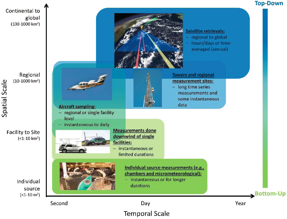
Atmospheric greenhouse gas (GHG) measurements are collected with a variety of techniques, including ground, aircraft, and satellite based, in order to capture the range of characteristics of GHGs. Some gases have very small horizontal and vertical gradients (i.e., CO₂), while others, which react more quickly in the atmosphere (e.g., methane), have substantial atmospheric gradients, both horizontally and vertically. For a gas like CO₂, on the one hand, small spatial gradients make it possible to generally characterize the global distribution with a small number of measurements across the globe. On the other hand, the fluxes of interest (e.g., changes due to a specific emission sector or source) create only small gradients, so it is critical that measurement techniques can sense small concentration gradients, especially in areas where emission and removal processes of interest are occurring. In order to observe GHGs across a range of spatial and temporal scales, a range of measurement techniques are used (Figure B-1) and described in detail in the following section.

Surface-based observations

In situ (i.e., continuous) ground measurements of atmospheric GHGs started with CO₂ in 1958 at the Mauna Loa observatory, Hawaii. This dataset, known as the reference CO₂ time series or “Keeling Curve” (Keeling et al., 1976), helped to determine CO₂ growth rate and trends and the rapid increase of global atmospheric CO₂. This increase is attributed to the accumulation of about half of anthropogenic CO₂ emissions in the atmosphere (Friedlingstein et al., 2019). Since then, many in situ measurement stations have been developed to improve understanding of the variability and trends of GHG emissions and carbon sinks at different scales. Information about global and regional measurement networks is managed by the World Data Centre for Greenhouse Gases (WDCGG) program.¹ The World Meteorological Organization (WMO) is responsible for international GHG calibration scales, which are deployed on all stations reporting to the WDCGG

___________________

¹https://gaw.kishou.go.jp/

program. Most stations measure in situ CO₂, methane (CH₄), and N₂O, and, in some cases, monitor SF₆ and F gases.

The global in situ GHG network is currently composed of 32 stations located in remote locations to monitor the representative large-scale trends not influenced by major local sources of atmospheric CO₂, CH₄, N₂O, SF₆, and fluorinated gases in both hemispheres, and to infer information on the latitudinal distribution of sources and sinks.² Most stations are equipped with meteorological sensors and some are also instrumented to monitor emission tracers (e.g., Radon-222, carbon isotopes, carbon monoxide [CO], oxygen) used as tools for partitioning anthropogenic versus natural fluxes (Ciais et al., 1995; Tans et al., 1990) and separating oceanic versus continental fluxes (Battle et al., 2000; Keeling et al., 1996). The U.S. National Oceanic and Atmospheric Administration (NOAA) deployed stations on a north-to-south gradient at four baseline observatories: Utqiaġvik (formerly Barrow), Alaska; Mauna Loa, Hawaii; American Samoa; and South Pole, Antarctica.³

___________________

² The initial sites were placed in remote locations far from anthropogenic emissions sources to provide a more accurate measure of the trends in well-mixed, long-lived GHGs. This siting, however, limits the ability of these stations to precisely identify specific sources of emissions, as was found in the case of “unexpected” CFC-11 emissions (Montzka et al., 2018).

³https://gml.noaa.gov/ccgg/insitu/#:~:text=NOAA%20Baseline%20Observatories&text=GML%20measures%20greenhouse%20gases%20at,CO%20measurements%20in%20the%201980’s

Other countries then joined the global in situ GHG network including Canada, China, Japan, Australia, and various European countries. The global CO₂ datasets are used to constrain global inversion models (e.g., Bousquet et al., 2000; Denning et al., 1995; Fernández-Martínez et al., 2019; Rayner et al., 2008) and assimilation systems such as CarbonTracker,⁴ Copernicus Atmosphere Monitoring Service (e.g., Pinty et al., 2019), and the National Aeronautics and Space Administration’s (NASA’s) Goddard Earth Observing System (GEOS) (Weir et al., 2021).

Continental GHG networks.

Continental networks have been developed over the last two decades to better assess trends and variability of atmospheric GHG concentrations, sources, and sinks at the regional to continental scales. Continental networks are also used to detect trends in atmospheric GHGs (e.g., Ramonet et al., 2010) to constrain inverse modeling frameworks (e.g., Monteil et al., 2020), and to study the impact of climate events on natural ecosystems, such as drought events (e.g., Smith et al., 2020). These networks monitor atmospheric GHGs in the lower atmosphere (i.e., continental boundary layer and the free troposphere) with stations deployed on tall towers or on top of mountains and far from local sources to ensure a regional representativeness of each site.⁵ The sites are equipped with meteorological sensors, which provide key ancillary datasets such as wind speed and direction to analyze atmospheric GHG variability (Yver-Kwok et al., 2021). Some sites are also equipped with remote sensing instruments (e.g., lidar, ceilometers) and make measurements of other gases (e.g., CO) that can be used to identify anthropogenic versus natural fluxes (e.g., Palmer et al., 2006).

In Europe, the GHG continental in situ network, ICOS-Atmosphere (Integrated Carbon Observing System⁶), has been operational since 2012 and includes about 50 in situ stations. Each country operates its own network and the data are sent every day and integrated into one central database with harmonized protocols (Hazan et al., 2016). The datasets feed the European Copernicus GHG assimilation system.⁷ In the United States, the continental network is managed by NOAA and started in the 1990s.⁸ All sites are equipped with tall towers with standardized instrumentation, and a central datacenter, and are linked to the international WMO GHG calibration scales. The NOAA tall tower network is part of the North American Carbon Program and its datasets used as a primary input for NOAA’s Carbon Tracker CO₂ and methane data assimilation systems.

National GHG networks.

National GHG networks are partly embedded into continental networks, for example in Europe and in the United States, and used to assess GHG emissions at the national scale. Several studies assessed emissions inventories independently through atmospheric observation-based methods, as detailed in Chapter 2.

Urban GHG networks.

Since the 2010s, urban GHG networks have been developed to better quantify emissions and understand uncertainty at these scales. Such measurements address mostly CO₂ across all sectors; although urban emissions are often dominated by energy consumption in the building and transportation sectors, some “producer” cities have considerable emissions in the industrial sector. Efficient urban measurements are designed with sites deployed in both dominant upwind and in-path or downwind locations with background regional sites upwind of the city and sites downwind of the city. Urban atmospheric GHG enhancements are then determined by subtracting the data collected at the background sites from the data collected at the urban sites. Additional measurements of emission tracers such as CO, nitrogen oxides (NO_x), volatile organic compounds (VOCs), and carbon isotopes can be key tools to partition fossil vs modern fluxes and to discrimi-

___________________

⁴https://gml.noaa.gov/ccgg/carbontracker

⁵https://www.icos-cp.eu/observations/atmosphere/stations

⁶https://www.icos-cp.eu

⁷https://atmosphere.copernicus.eu/ghg-services

⁸https://gml.noaa.gov/ccgg/insitu/#:~:text=NOAA%20Baseline%20Observatories&text=GML%20measures%20greenhouse%20gases%20at,CO%20measurements%20in%20the%201980’s

nate source categories (e.g., Ammoura et al., 2016; Graven et al., 2018). Ancillary meteorological parameters are necessary to interpret atmospheric GHG variability (e.g., Xueref-Remy et al., 2018).

Several intensive urban measurement efforts have been deployed in recent years, starting in 2010 with the INFLUX project in Indianapolis (Turnbull et al., 2015), the MEGACITIES project in the Los Angeles megacity (Verhulst et al., 2017), and the CO₂-MEGAPARIS project in the Paris megacity (Xueref-Remy et al., 2018). Other urban intensives that have been developed since then include the Northeast United States corridor from Boston to Washington, DC (Karion et al., 2020), Salt Lake City (Lin et al., 2018; Mitchell et al., 2018), São Paulo, Brazil (Pérez-Martínez et al., 2020), Tokyo, Japan (Imasu and Tanabe, 2018), Aix-Marseille, France (Xueref-Remy et al., 2020b), and other European cities as a test bed of the ICOS cities project.⁹ The WMO Integrated Global Greenhouse Gas Information System (IG³IS) scientific community recently published a first report on urban network design recommendations.¹⁰ Systemic urban GHG measurements are still rare in the Global South.

Mobile in situ measurements.

Mobile in situ measurements (e.g., using a car or train platform) bring additional information to in situ urban measurements, particularly on characterizing GHG spatial variability (Idso et al., 2001; Mallia et al., 2020). Mobile campaigns in urban areas are also used to infer methane sources in cities, mostly from leaking gas lines (Carranza et al., 2022; Phillips et al., 2013; Xueref-Remy et al., 2020a).

Eddy covariance (EC) flux measurements.

Eddy covariance is a technique based on the principle of atmospheric turbulence, which measures GHG fluxes (mostly CO₂ and CH₄) from high-frequency GHG concentrations and 3D wind measurements. Measurements are usually done on a mast several meters above the canopy of buildings/vegetation or in an open-view area to avoid perturbations from surrounding structures/trees. The footprint of the EC measurements is usually determined from atmospheric dispersion models or analytical solutions of the diffusion equation (e.g., Kljun et al., 2015). Typically, the footprint of an EC station is a hundred square meters to some square kilometers (Rebmann et al., 2018). While most often deployed on natural areas, the EC approach has recently been used in some cities to assess urban CO₂ and methane emissions, for example in the center of London (Helfter et al., 2016), Helsinki (Järvi et al., 2012), and Florence (Gioli et al., 2015).

EC flux measurement sites have been mostly developed starting in the 1990s to assess local, regional, national, and continental fluxes and were further organized into networks within large and long-term observation infrastructures, for example in Europe (ICOS-Ecosystems¹¹) and in the United States (FLUXNET;¹² NEON;¹³ AMERIFLUX¹⁴). Over the last decade, some EC stations were deployed to assess urban CO₂ and CH₄ emissions and to independently verify local emissions inventories (e.g., Helfter et al., 2016). Such measurements were also used to assess the impact of the COVID-19 lockdown on CO₂ emissions. For example, an EC study conducted in 11 European cities estimated a reduction of 5 to 87 percent of urban CO₂ emissions during that period, mostly from a decrease in traffic (Nicolini et al., 2022).

Point-source in situ measurements.

Point-source in situ measurements have been performed to improve estimates of anthropogenic GHG sources and emissions. Point-source measurements of methane from mobile campaigns have been used mainly for (1) detecting methane gas leaks (e.g., Keyes et al., 2020); (2) identifying methane point sources (e.g., Zazzeri et al., 2015); and (3)

___________________

⁹https://www.icos-cp.eu/projects/icos-cities-project#:~:text=ICOS%20Cities%20(PAUL%20%E2%80%93%20Pilot%20Applications,measurement%20system%20for%20urban%20areas

¹⁰https://ig3is.wmo.int/en/news/towards-international-standard-urban-ghg-monitoring-and-assessment

¹¹https://www.icos-cp.eu/observations/ecosystem/etc

¹²https://fluxnet.org

¹³https://www.neonscience.org/about

¹⁴https://ameriflux.lbl.gov

quantifying methane source emissions (e.g., Yacovitch et al., 2015). Such campaigns have been widely developed in several countries in the last decade due to the large underestimation of methane emissions. Point-source measurements allow an independent assessment of methane sources given by regional and national inventories and reveal missing or underestimated sources (e.g., Al-Shalan et al., 2022; Marklein et al., 2021; Varon et al., 2019; Xueref-Remy et al., 2020a). Point-source measurements have also been used to assess fossil fuel CO₂ emissions, for example, by sampling transects across an industrial CO₂ source plume stripped from natural gas and vented to the atmosphere in New Zealand (Turnbull et al., 2014).

Ground-based remote sensing.

There is a long history of using open path Fourier transform spectroscopy (OP-FTIR) measurements to characterize atmospheric gases, generally at the facility scale with commercially available measurement systems. More recent research has expanded this to use ultraviolet and visible light, and, more recently, near-infrared light (Griffith et al., 2018). Recent innovations led to CO₂ and methane measurements over distances of 1.5 km with improvements in measurement repeatability and reduced bias, extending the application of this technique from the industrial scale to city scale. Specific plumes can be detected, and in some cases quantified, with commercial and thermal infrared (Ravikumar et al., 2017) and in research work with stationary hyperspectral cameras using shortwave infrared (Knapp et al., 2022).

Uplooking FTIR measurements have been deployed in a global validation network utilized by the satellite community. This technique relies on direct sun measurements at (near infrared) wavelengths to characterize to total atmospheric column a wide range of trace gases. The data are used for scientific investigations as well as satellite validation. The Total Carbon Column Observing Network (TCCON) uses a Bruker FTIR, Suntracker, and is typically housed in a shipping container. The TCCON sites are periodically overflown by aircraft or Aircore to establish a connection between the uplooking data and the standards used with in situ measurements. A more portable, lower cost instrumentation approach has been developed using the EM-27 spectrometer (Gisi et al., 2012). These are being deployed in research networks in Berlin (Rißmann et al., 2022), Toronto (Mostafavi Pak et al., 2019), Namibia (Frey et al., 2021), and Uganda (Humpage et al., 2020) and in a new validation network, COCCON (COllaborative Carbon Column Observing Network) (Frey et al., 2019).

Aircraft-based observations

Aircraft in situ measurements.

Regular commercial aircrafts have been used as scientific platforms for monitoring atmospheric GHGs in the troposphere and at the upper troposphere/lower stratosphere levels; such programs have been developed in the 1980s in Japan (CONTRAIL; Matsueda et al., 2002, 2008) and then by Germany as the CARIBIC (Civil Aircraft for the Regular Investigation of the atmosphere Based on an Instrument Container) flying observatory,¹⁵ further completed in the 2010s by several European countries within the IAGOS Research Infrastructure.¹⁶ Urban networks do not exist in all cities, and airborne campaigns could be performed more regularly to provide emissions estimates and a regular independent assessment of emission inventories.

Aircraft remote sensing.

Aircraft remote sensing has been used widely for CO₂ and methane measurements, while other GHGs (e.g., N₂O, F gases) have not been sampled with aircraft remote sensing techniques. Some recent reports of measurements include the AVIRIS-NG (Airborne Visible-Infrared Imaging Spectrometer—Next Generation), PRISMA (PRecursore IperSpettrale della Missione Applicativa), and GAO (Global Airborne Observatory) sensors for CO₂ and methane measurements (Cusworth et al., 2021a, 2021b). The aircraft instrument MAMAP (Methane

___________________

¹⁵https://www.caribic-atmospheric.com/

¹⁶https://www.iagos.org/

airborne MAPper) has also been developed in support of the CO2M mission development and has been used to measure CO₂ (Krings et al., 2018) and methane (Krautwurst et al., 2021). GOBLEU¹⁷ (Greenhouse gas Observations of Biospheric and Local Emisions from the Upper sky) is an aircraft program jointly launched by Japan Aerospace Exploration Agency (JAXA) and All Nippon Airways (ANA). GOBLUE will collect CO₂ and NO₂ measurements from ANA commercial aircrafts and prototypes the combined use of CO₂ and NO₂ for better emissions monitoring.

Space-based observations

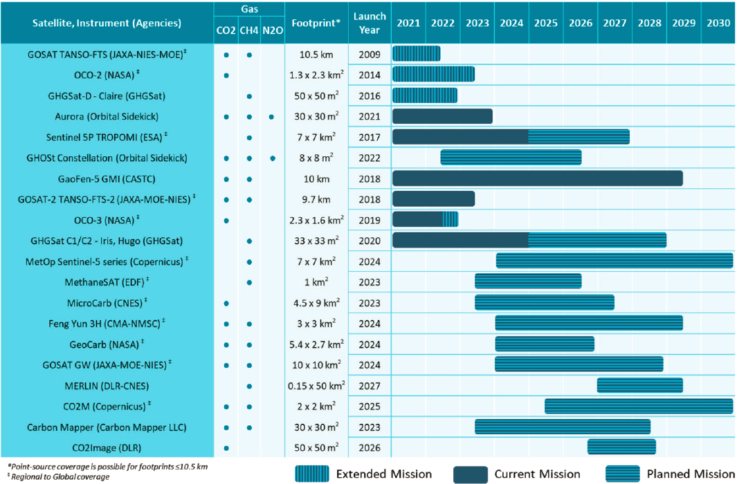
Major advances in satellite remote sensing of GHGs were made in the 2010s and 2020s. The evolution of measurements and roadmap for future missions are well described in reports such as CEOS (2018) and the European Commission’s CO₂ Reports (Ciais, 2015; Pinty et al., 2017, 2019) Satellite measurements (Figure B-2) have been used to quantify GHG emissions from power plants, observe enhancements from cities, and estimate fluxes from a wide set of regions of the world, as well as provide global overviews. As detailed in NASEM (2018), satellite measurements have evolved from large (30 km × 60 km for the SCIAMACHY experiment) footprint measurements. Footprint sizes were reduced in satellites that followed, including GOSAT (80 km²) and then TROPOMI (7 km × 7 km). Satellite measurements continue to improve in spatial and temporal resolution with the next generation of satellites (Figure B-2).

Multigas approaches and isotopic analysis

Isotopic analysis.

As radiocarbon (¹⁴C) is radioactive with a lifetime of ~5,730 years, ¹⁴C measurements in atmospheric CO₂ are used at the urban to the national scales to discriminate CO₂ emissions from the burning of fossil fuels (which do not contain any radiocarbon atoms) from modern CO₂ fluxes (i.e., from vegetation fluxes or wood burning) (Miller et al., 2012). ¹⁴C measurements of methane are rare because of the low signal to be detected, but emerging techniques are promising (Zazzeri et al., 2021). The ¹³C to ¹²C ratio depends on CO₂ sources and can be used to discriminate different sources of CO₂ and methane through Keeling plot or Tans-Miller plot methods, especially for urban CO₂ (e.g., Lopez et al., 2013; Zazzeri et al., 2021) and point sources—mostly through mobile campaigns—for methane (e.g., Al-Shalan et al., 2022; Xueref-Remy et al., 2020a). Isotopic information can be compared to emission inventories and used to improve source characterization (e.g., completeness, location, intensity). Both ¹⁴C and ¹³C methods have been used at the global scale to quantify the impact of the increasing burden of anthropogenic emissions on atmospheric CO₂ since the pre-industrial era.¹⁸

Tracer to tracer approach.

Most GHG observation programs combine in situ CO₂ measurements with emission tracers (e.g., non-methane volatile organic compounds [NMVOCs], CO, NO_x, black carbon [BC], sulfur oxides [SO_x]) collected by research institutes or air quality agencies. These emission tracers can be used to discriminate between emission sources by analyzing correlations and ratios between CO₂ and the emission tracers. Most combustion processes are incomplete, producing not only CO₂ but other species such as CO, NO_x, VOCs, BC, and SO_x. Some species are typical of some sources—for example, NO_x and isopentane are often attributed to traffic, ethane and butane are more associated with natural gas heating, and SO_x is more associated with combustion of sulfur-containing fossil fuels such as coal in electricity generation and diesel or heavy fuel oils used in transport and shipping. BC mixing ratios peak depending on the absorption wavelength of BC particles and can be attributed either to wood burning or to fossil fuel burning sources.

___________________

¹⁷https://www.eorc.jaxa.jp/GOSAT/ANAexp/index_e.html

¹⁸https://gml.noaa.gov/ccgg/isotopes/c13tellsus.html

Analyzing the correlations and ratios between CO₂ and these tracers, especially in concomitant mixing ratio CO₂-tracer peaks, especially at key time periods such as rush hour and domestic heating, is a method often used to identify the different sources of CO₂ and their temporal variability (e.g., Lopez et al., 2013). This method has highlighted inaccurate emission ratios between emission tracers and CO₂ in inventories, improving emission ratios and source partitioning in urban to national inventories (e.g., Ammoura et al., 2016). Methane is also co-emitted with other species, such as ethane, which is one component of natural gas. Ethane-to-methane correlations have been used to estimate fugitive methane emissions from urban centers (Plant et al., 2019) and revealed an underestimation of methane emissions in the inventories of these cities. It is worth noting that using a single value for ethane-to-methane ratios—for example, for the entire oil and gas supply chain—can introduce significant errors into source attribution (Allen, 2016).

Dual tracer approaches can be used to calculate methane emissions at point sources, such as landfills, natural gas storage sites, wastewater treatment facilities, and cattle farms, by releasing a tracer such as acetylene (due to its negligible background level) at the methane source location at a known emission rate. The measured ratio of methane to a tracer downwind of the source plume, combined with the known tracer emission rate, provides a quantification of the methane emission rate and delivers an independent estimate of methane emissions of that source from the inventory. This approach can be used to improve emissions inventories (e.g., Roscioli et al., 2015; Vechi et al., 2022; Zavala-Araiza et al., 2018).

Radon-222 is a natural tracer emitted by the continental crust with a lifetime of 3.8 days, typical of the synoptic scale. Its emission rate varies with the nature of soils and is available in the literature for different continental surfaces. Concomitant atmospheric measurements of radon-222 and GHGs are used with a known Rn-222 flux and the air mass footprint (i.e., the surface seen by the air mass before reaching the measurement site) from wind measurements to calculate GHG emissions at the regional scale. Such results help to assess independent regional and national inventories for species such as CO₂ and N₂O (e.g., Schmidt et al., 2001, 2003; Xueref-Remy et al., 2020b).