
2
Current Approaches for Quantifying Anthropogenic Greenhouse Gas Emissions
Greenhouse gas (GHG) inventories are tools that quantify GHG emissions (or removals) often divided into economic and industrial sectors over a specific time period. They are most often resolved to the nation, province, or city scale but can also be resolved down to individual emitting infrastructure (e.g., facilities, buildings, roads), or aggregated over multiple facilities across geographies or jurisdictional boundaries. Many global inventories are spatially resolved to regular “gridded” form, a common practice at the global scale, allowing for integration with atmospheric modeling systems. GHG inventories typically span multiple years, with annual resolution, but many will resolve to finer temporal scales such as month, day, or hour. GHG inventories are developed and used by a range of stakeholders including policy makers (at multiple scales), the scientific community, businesses, media, nongovernmental organizations (NGOs), and the general public. By quantifying GHG sources and sinks, GHG inventories can inform emission baselines or spatial distributions, track emission changes over time, and assess emission mitigation efforts for a specific entity over a period of time (Schaltegger and Csutora, 2012). Inventories can also form the basis of projections and future emission scenarios, further assisting with mitigation planning and tracking.
GHG inventories are constructed using a wide variety of approaches. Broadly, in this report, we classify them into three groups: (1) activity-based approaches, (2) atmospheric-based approaches, and (3) mixed or “hybrid” approaches. The Committee chooses not to use the more familiar “bottom-up” and “top-down” terminology. Activity-based approaches are most familiar to decision makers and have been most commonly deployed for decision making purposes. Atmospheric-based approaches have seen extensive development in the research community. While atmospheric-based approaches have had less application to decision-making, to date, increasingly their application to decision making is being discussed, often as a complement to activity-based approaches. Finally, mixed or hybrid approaches have seen only recent development, but offer a promising means to build more relevant and accurate inventories in the future. We describe each of these approaches below, noting source data, general methods, scope, and current examples.
Activity-Based Approaches
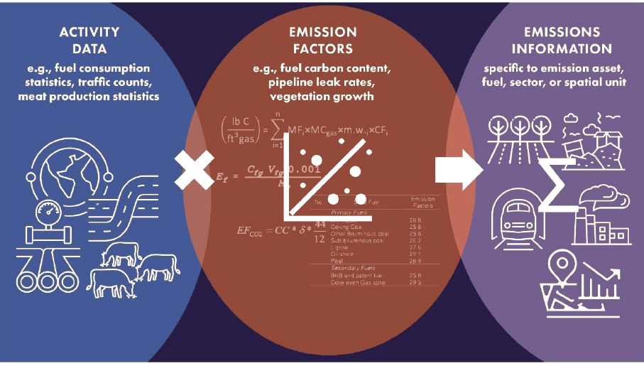
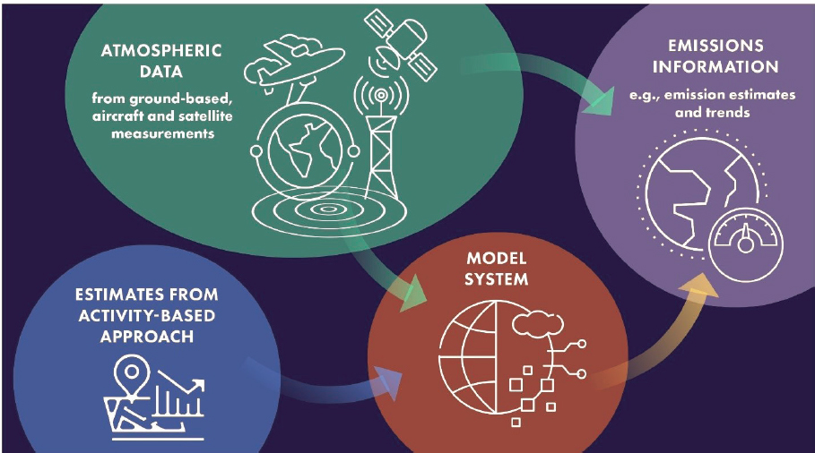
Activity-based approaches (often referred to as “bottom-up” approaches) encapsulate a wide variety of data sources and methods. The common element among the many activity-based GHG inventories is the general use of activity data, a term referring to representative indicators or drivers of GHG emissions within system (or model) boundaries, such as fuel consumption statistics, traffic counts, local air pollution quantities, population, or vegetative cover. The type of activity data employed in GHG inventory estimation efforts is often unique to the economic sector, technology, and the specific GHG. In this report, we also include direct flux monitoring such as a continuous emissions monitor (typically placed in an effluent stream), as part of activity-based approaches. Even though continuous emissions monitors measure gas concentrations, these are not considered traditional atmospheric measurements and require additional information (mass flowrate) to be used to estimate an emissions amount. Hence, they are grouped with activity-based (or other “bottom-up”) approaches in this report. By contrast, we consider eddy flux measurements, which incorporate atmospheric dynamics, part of atmospheric-based approaches.
To achieve an estimate of a GHG flux, these activity measures must be transformed using an “operator” or emission factor (a coefficient that represents the emission or removal of a GHG per unit of activity) (Figure 2-1).
This general approach is often represented in its simplest form as
| emissions = AD × EF | (1) |
where AD represents an activity measure and EF an emission factor. This simple representation (Equation 1) assumes that emission factors are constant and representative for a given activity for the duration of consideration. Specifically, activity-based approaches may fail to describe complex
processes such as emissions and removals associated with managed vegetation, unintended emissions or disruptive emissions (e.g., equipment failure, natural gas pipeline leaks), and wartime military activities that require more complex modeling constructs. Additionally, some emission factors are well characterized with measures of uncertainty (e.g., the carbon content of natural gas has been measured widely and its regional variation well understood), while others are either established from small samples or specific application settings and are poorly characterized or represent mean values (e.g., N2O from soils). Because activity-based approaches are most often sector, fuel, and technology specific, they comprise a mixture of both simple and more complex versions of Equation 1, and can incorporate direct flux monitoring.
Production (Direct) Versus Consumption (Indirect) Perspectives
GHG inventories can be expressed as “production” (i.e., direct) or “consumption” (i.e., indirect) inventories, depending on how the system boundary is defined for the GHG accounting problem (Peters, 2008). Production inventories tie emissions to the geographic location where they enter the atmosphere (Figure 2-2). These emissions are often also referred to as “Scope 1” emissions, a term that emanates from the language originating with corporate and organizational GHG accounting (WRI/WBCSD, 2004). The consumption-based GHG perspective refers to emissions that occur as a result of consumptive activity, much of which may occur in geographically distant locations outside of an entity’s territorial boundary. Therefore, consumption emissions incorporate emissions associated with the supply chain for all goods and services (often referred to as “Scope 3” emissions; Figure 2-2) and may employ, for example, life-cycle accounting techniques to quantify emissions (Chen et al., 2019). Although this approach is often thought of as incorporating “upstream”
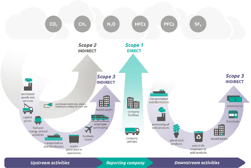
emissions, it also reflects “downstream” activities such as waste production, transport to landfill or combustion locations, and end use of a product. Scope 2 emissions are specifically related to the assignment of GHG emissions from electricity, heat, or steam production from a power plant to the point of consumption (e.g., household, office building, factory; Figure 2-2).
The distinction between Scope 1 versus Scope 2 and 3 accounting perspectives tends to be a more critical consideration as the spatial scales decrease. The accounting perspective is also critically important when considering approaches to quantify GHGs. For example, because atmospheric-based approaches only “see” emissions from the Scope 1 or production perspective, incorporating atmospheric-based approaches with consumption-based GHG accounting can be challenging to integrate.
Survey of Current Global/National Activity-Based GHG Inventories
Many activity-based GHG inventories have been developed over the past four decades. We first distinguish a hierarchy for describing these GHG inventories. We consider four size classes: (1) global/national, (2) national/regional, (3) local/urban, and (4) facility (see also Chapter 1) and their activity-based approaches below. The Statement of Task for this report focuses on the development of an evaluation framework for GHG information at the global/national scale, but here we provide a more complete general description across the scales currently considered in GHG emissions information efforts to provide context and useful case study examples.
UNFCCC GHG Inventories
The United Nations Framework Convention on Climate Change (UNFCCC) established the need for GHG emissions information at the global/national scale by requiring national governments to regularly report inventories. Participating Parties have employed the Intergovernmental Panel on Climate Change (IPCC) 1996 and 2006 guidelines in the preparation and submission of these inventories (IPCC, 2006; UNFCCC, 2014). Recognizing the limited institutional capacity of various countries in addressing methodological complexities, the IPCC guidelines specify a “tiered” GHG estimation approach (i.e., Tier 1, 2, 3) in which the complexity and presumed accuracy increase from Tier 1 to 3. The aim is to create inventories that are “Transparent, Accurate, Complete, Consistent, Comparable, and efficient in resource use” (IPCC, 2006). Tier 1 defaults generally involve the use of country-average data, while Tiers 2 and 3 involve more refined or granular estimation methods. In general, the IPCC emissions inventory estimation methods involve the use of activity data and corresponding emissions per unit of activity (Rypdal et al., 2006). The UNFCCC reporting process is summarized in Figure 2-3.
Under the Paris Agreement, all signatories are required to employ the Enhanced Transparency Framework (ETF)1 by 2024 to report, in a uniform basis, national GHG inventories and support collective evaluation efforts, including the every 5-year Global Stocktake (Box 2-1; see also Case Study 4.1). The ETF incorporates capacity considerations of developing countries while aiming to avoid undue burdens on the Parties (UNFCCC, 2020).2 The Capacity-building Initiative for Transparency provides support to developing countries’ commitments under the ETF, including the development of national inventories. Under the ETF process, all inventories will undergo review by
___________________
1 The ETF was established by Article 13 of the Paris Agreement.
2 Developed countries are required to report seven gases (CO2, CH4, N2O, HFCs, PFCs, SF6, and NF3). Developing countries that need flexibility due to their capacity level are required at a minimum to report emissions of CO2, CH4, and N2O, and any of the “F gases” (HFC, PFC, SF6, and NF3) if included in the Party’s nationally determined contributions (NDCs) or if they have F gases under Article 6 or previously reported them (UNFCCC, 2019, para. 48). Parties should report international aviation and marine fuel bunker emissions and should not include those emissions in national totals.
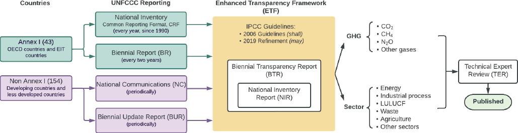
a group of technical experts to ensure reporting is consistent with international rules. Parties will track progress toward their country’s nationally determined contributions (NDCs)—non-binding national plans that include climate mitigation, adaptation, and financing commitments (including climate-related targets for GHG emission reductions)—before the publication of reports.
Global/national GHG Inventories
Beyond UNFCCC inventory reporting, many national/global GHG inventories have been developed with varying characteristics. For example, all the energy-related carbon dioxide (CO2) emissions in various datasets rely on energy statistical data from a small number of energy-reporting sources (Figure 2-4). The major four energy data archiving agencies (Energy Information
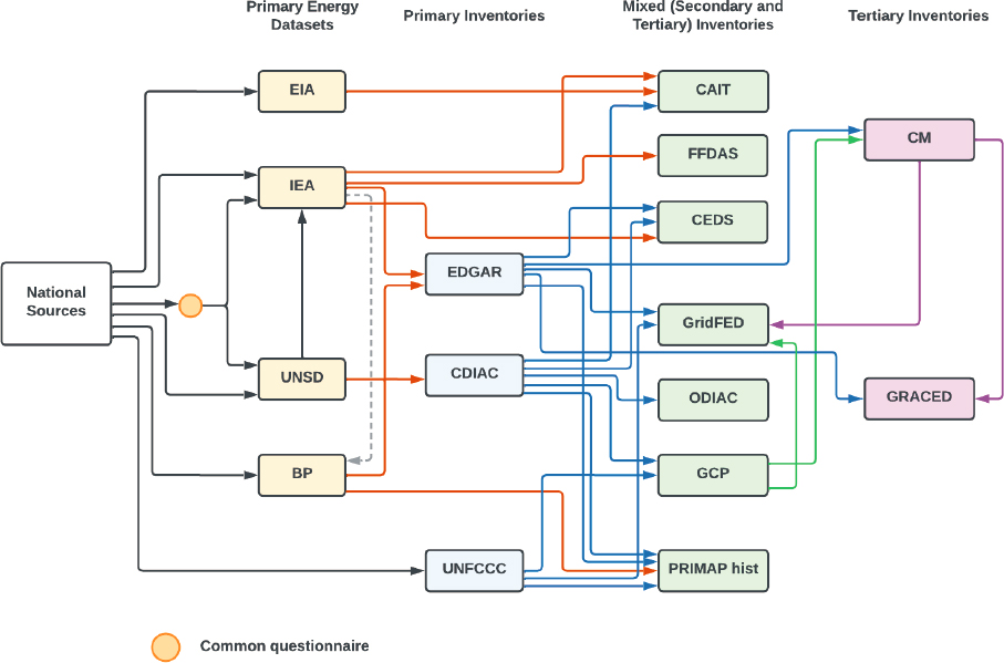
Administration, International Energy Agency, United Nations Statistics Division, and BP) in turn derive, in whole or part, energy consumption statistics from national sources in the form of questionnaires or surveys (Andres et al., 2012; Andrew, 2020). On the one hand, these efforts provide global data in a consistent manner; on the other hand, many of the energy data lack transparency due to confidentiality or intellectual property restrictions. This is a critical element in understanding the content of global/national inventories and in considering what independent information might be considered to evaluate and validate outcomes from the many global/national GHG inventories that use these source data. Primary inventories have been compiled globally that may combine two or more of the energy datasets to generate estimates of GHG emissions. There are a number of “mixed secondary/tertiary” inventories that use a mixture of primary energy/emissions data but also draw critical information from primary inventories. Finally, tertiary GHG inventories are primarily derived from primary inventories and typically provide additional space/time resolution (mostly through downscaling) or specific data additions.
It is important to note that the datasets listed in Figure 2-4 and Table 2-1 do not represent an exhaustive accounting of all global energy-related inventories. The goal of Figure 2-4 and Table 2-1 is to trace the relationship between national energy datasets and global inventories that utilize energy (and in some cases GHG emissions) information from those sources. While Figure 2-4 was modified from Andrew (2020), it does not adopt the same categories. This figure does not capture the details of individual inventories (e.g., timeliness of energy data updates), and the spatial resolution of each inventory is noted in Table 2-1.
For non-CO2 emissions, in addition to the sources listed in Table 2-1, the U.S. Environmental Protection Agency (EPA) produces national inventories using IPCC default methodologies, international statistics for activity data, and IPCC Tier 1 default emission factors (EPA, 2019). Methane (CH4) and nitrous oxide (N2O) specific inventories have also been developed at the global and national scale using activity-based approaches for projections of mitigation potential (e.g., Harmsen et al., 2019; Höglund-Isaksson et al., 2020). The Food and Agriculture Organization of the United Nations is a key source of activity data for land use and agricultural emissions.
Because CO2 emissions from the land use, land-use change, and forestry (LULUCF) sector use singular data and methods, they are often not incorporated into most of the global/national GHG inventories except in a few instances (e.g., Global Carbon Project, an annual summary report with their own gridded inventory; UNFCCC). However, several inventories specific to LULUCF sector emissions have been created (Table 2-1). Key distinctions among these global/national GHG inventories are whether the dataset includes carbonate sources (e.g., cement calcining), non-CO2 GHGs, net anthropogenic biosphere CO2, or industrial process/fugitive emissions (Table 2-1). Furthermore, some inventories separate agriculture and LULUCF while others combine them into a single sector (agriculture, forestry, and other land use [AFOLU]), making comparability challenging. There are also distinctions in how the information output is categorized and reported (e.g., whether the output is at subnational or subannual scales, the resolution, latency, amount of sector detail). Finally, there are distinctions in methodologies associated with emission factors and/or modeling differences (e.g., for net anthropogenic biosphere CO2).
The energy-related global GHG inventories listed in Table 2-1 all reflect a Scope 1 or territorial accounting perspective. However, global GHG inventories that reflect a Scope 3 or consumption perspective have been developed, though this has been primarily at country resolution (e.g., Davis and Caldeira, 2010; Hertwich and Peters, 2009; Kanemoto et al., 2016; Moran et al., 2018). Consumption-based GHG emissions are included in the inventory development of the Global Carbon Project (Friedlingstein et al., 2022).
TABLE 2-1 National or Global Greenhouse Gas Inventories and Key Characteristics
| Inventory Name | Gases | Geographic coverage | Resolution (space, time) | Time period (latency) | Sectors (yes/no) | Cement (yes/no) | Fuel type (yes/no) | Reference | Webpage |
|---|---|---|---|---|---|---|---|---|---|
| PRIMARY ENERGY DATASETS | |||||||||
| International Energy Agency (IEA) | Energy, CO2, CH4 | 190 countries | Country, annual | 1971–2020 1960–2020 (OECD) | Yes | No | Yes | IEA, 2021a,b | https://www.iea.org/data-and-statistics/data-products |
| Energy Information Administration (EIA) | Energy, CO2 | 230 countries | Country, annual | 1980–2019 (country) 1949–2018 (global) | No | No | Yes | EIA, 2021 | https://www.eia.gov/environment/emissions/state/ |
| BP | Energy, CO2 | 80 individual countries, 12 regional aggregates | Country/region, annual | 1965–2021 | No | Yes | Yes (energy), No (emissions) | BP, 2022 | https://www.bp.com/en/global/corporate/energy-economics/statistical-review-of-world-energy.html |
| UN Statistics (UNSD) | Energy, CO2 | 230 countries/territories | Country, annual | 1990–2020 (publicly available) | No | No | Yes | Pachauri et al., 2014 | https://unstats.un.org/unsd/energystats/data/ open data: http://data.un.org/Explorer.aspx |
| PRIMARY INVENTORIES | |||||||||
| United Nations Framework Convention on Climate Change (UNFCCC) | CO2, CH4, N2O, CO, NMVOC, SO2, HFCs, PFCs, SF6, NF3, CO2-LULUCF | All Parties | Country, Annex I: annual, non-Annex I: biennial | 1990–2020 (T-2) (developed) or 1990–various (T-4) (developing) | Yes | Yes | Yes | UNFCCC, 2021a | https://unfccc.int/process-and-meetings/transparency-and-reporting/greenhouse-gas-data/ghg-data-unfccc/ghg-data-from-unfccc |
| Emissions Database for Global Atmospheric Research (EDGAR) | CO2, CH4, N2O, F-gases (HFC, PFCs, SF6, NF3), Air pollutants (SO2, NOX, NMVOC, CO, NH3, PM2.5, PM10, BC, OC) | 228 countries, global | 0.1°×0.1°, monthly | 1970–2018 (NA) | Yes | Yes | No | Crippa et al., 2021 | https://edgar.jrc.ac..europa.eu/report_2021 |
| Carbon Dioxide Information Analysis Center (CDIAC) | CO2 | 259 countries | Country, annual | 1751–2017 | No | Yes | Yes | Gilfillan and Marland, 2021 | https://cdiac.ess-dive.lbl.gov/ |
| Gridded Global Model of City Footprints (GGM-CF) | CO2 (consumption-based footprint) | 13,000 cities | Urban area | 2013 | No | Yes | No | Moran et al., 2018 | https://www.citycarbonfootprints.info/ |
| MIXED SECONDARY/TERTIARY INVENTORIES | |||||||||
| Global Carbon Project (GCP) | CO2, CO2-LULUCF (also consumption-based CO2) | 259 countries (FFCO2 only) | Country, annual | 1750–2020 (FFCO2) 1850-2020 (LULUCF) | Yes | Yes | Yes | Friedlingstein et al., 2022 | https://www.globalcarbonproject.org/carbonbudget/ |
| Fossil Fuel Data Assimilation System (FFDAS) | CO2 | 137 countries, 3 regional aggregates | 0.1°×0.1°, monthly | 1997-2015 | No | No | No | Asefi-Najafabady et al., 2014 | https://ffdas.rc.nau.edu/Data.html |
| Community Emissions Data System (CEDS) | SO2, NO2, BC, OC, NH3, NMVOC, CO, CO2, CH4, N2O | 221 countries | 0.5°× 0.5°, monthly | 1750–2019 1970–2019 (CH4 and N2O) | Yes | Yes | No (only global) | Hoesly and Smith, 2018; McDuffie et al., 2020; O’Rourke et al., 2021 | http://www.globalchange.umd.edu/ceds/ |
| Potsdam Real-time Integrated Model for probabilistic Assessment of emissions Paths (Primap-Hist) | CO2, CH4, N2O, F-gases, HFCs, PFCs, SF6, NF3 | All UNFCCC member states, most non-UNFCCC territories | Country, annual | 1750–2019 | Limited | Yes | No | Gütschow et al., 2019 | https://www.pik-potsdam.de/paris-reality-check/primap-hist/ |
| CAIT/Climate Watch | CO2, CH4, F-gases, N2O | 185 countries | Country, annual | 1850–2019 (country) 1990–2019 (sectors) | Yes | Hennig et al., 2017 | https://www.climatewatchdata.org/ | ||
| Inventory Name | Gases | Geographic coverage | Resolution (space, time) | Time period (latency) | Sectors (yes/no) | Cement (yes/no) | Fuel type (yes/no) | Reference | Webpage |
|---|---|---|---|---|---|---|---|---|---|
| Open-source Data Inventory for Anthropogenic CO2 (ODIAC) | CO2 | 259 countries | 1km×1km, monthly | 2000–2019 | Partial | Yes | Yes | Oda et al., 2018 | https://db.cger.nies.go.jp/dataset/ODIAC/ |
| GCP-GridFED | CO2 | 259 countries | 0.1°×0.1°, annual | 1959–2018 | Yes | Yes | Yes | Jones et al., 2021 | https://mattwjones.co.uk/co2-emissions-gridded/ |
| TERTIARY EMISSIONS | |||||||||
| Carbon Monitor | CO2 | 6 countries, EU+UK, ROW | Country and region, 0.1°×0.1°, daily | 2019–2022 | Yes | Yes | No | Liu et al., 2020a | https://carbonmonitor.org/ |
| Global Gridded Daily CO2 Emissions Dataset (GRACED) | CO2 | 6 countries, EU+UK, ROW | 0.1°×0.1°, daily | 2019–2020 | Yes | Yes | Dou et al., 2022 | ||
| LULUCF/AFOLU | |||||||||
| FAOSTAT | CO2, CH4, N2O, CO2-LULUCF | 1961–2019 | Yes | NA | NA | Tubiello et al., 2013 | https://www.fao.org/faostat/en/ | ||
| BLUE | CO2-LULUCF | Global | 0.25°×0.25°, annual | 1700–2019 | No | NA | NA | Hansis et al., 2015; updated simulations described by Friedlingstein et al., 2020 | |
| OSCAR | CO2-LULUCF | 10 regions | Regions, annual | 1701–2019 | No | NA | NA | Gasser et al., 2017; 2020; Friedlingstein et al., 2020 | https://www.icos-cp.eu/science-and-impact/global-carbon-budget/2020 |
| H&N | CO2-LULUCF | 187 countries | Country, annual | 1850–2019 | No | NA | NA | Friedlingstein et al., 2020; Houghton and Nassikas, 2017 |
NOTES: The efforts presented here attempt to capture the most established, commonly used greenhouse gas (GHG) inventories published in the peer-reviewed literature. It is not exhaustive of all global GHG inventories, particularly those under development, and contains a mixture of gridded and non-gridded inventories. CO2, carbon dioxide; CH4, methane; N2O, nitrous oxide; CO, carbon monoxide; NMVOC, non-methane volatile organic compound; SO2, sulfur dioxide; F-gases, fluorinated gases; HFCs, hydrofluorocarbons; PFCs, perfluorochemicals; SF6, sulfur hexafluoride; NF3, nitrogen trifluoride; BC, black carbon; OC, organic carbon; NO2, nitrogen dioxide; NOx, nitrogen oxides; PM, particulate matter; NH3, ammonia; FFCO2, fossil fuel CO2; CO2-LULUCF, CO2 from land use, land-use change, and forestry; LULUCF, land use, land-use change, and forestry; AFOLU, agriculture, forestry, and other land use; T, current year; EU, European Union; UK, United Kingdom, ROW, rest of world; OECD, Organisation for Economic Co-operation and Development.
SOURCE: Modified from Andrew, 2020 and Minx et al., 2021.
Regional/national GHG Inventories
Here we consider a separate scale of GHG inventories that span regional (multistate/province) to subnational (~provincial/state scale—larger than the local/urban scale) to national domains. They are relevant at the global scale as they provide some GHG inventory examples with features and innovations that are worth considering when evaluating the strengths and weaknesses of the global/national GHG inventories. We provide examples of these efforts in Box 2-2 and below to illuminate the approaches, innovations, and opportunities they offer.
China has quantified emissions in multiple ways, with subnational granularity, unique datasets, and detailed sector composition (e.g., Guan et al., 2012; Liu et al., 2015; Shan et al., 2020) (see also Case Study 4.2). The Multiresolution Emission Inventory for China—High Resolution (MEIC-HR) emissions data product merges county/provincial resolution nonpoint sources with a detailed database of factory and power plant emissions sources; point sources are quantified from facility-scale fuel consumption statistics (Zheng et al., 2021). A comprehensive comparison of different activity-based inventories has been performed by Han et al. (2020).
Notable in the United States and the United Kingdom are efforts to quantify consumption-based emissions at subnational scales (Jones and Kammen, 2015; Minx et al., 2013). Such efforts rely on economic consumption statistics and downscaling through divisions of economic activity into commodity categories. There is also a wider array of efforts aimed at individual process or individual GHGs at the regional/national scale. For example, Maasakkers et al. (2016) produced a methane emissions inventory for the United States based on the combination of numerous datasets. Similarly, over a dozen activity-based studies were conducted in the United States across the natural gas supply chain employing ground-based methods such as the use of tracer-flux, direct measurements such as high-flow sampling, calibrated bags, and mobile measurement techniques (Allen et al., 2013; Brantley et al., 2014; Lamb et al., 2015; Mitchell et al., 2015; Subramanian et al., 2015; von Fischer et al., 2017). The EPA also produces global non-CO2 emissions inventories at the national scale in approximately annual reports (e.g., EPA, 2019, 2022).
Local/urban GHG Inventories
Considering the local/urban scale in an evaluation framework for GHG inventories is relevant because efforts at these scales demonstrate valuable attributes—including granularity and completeness—that make them more usable and relevant for decision makers. Approaches used at the local/urban scale could be scaled to larger jurisdictions and thereby enrich the suite of techniques at the global/national scale.
Local/urban GHG inventories are produced for a large portion of cities around the globe. For example, 9,120 cities representing over 770 million people (10.5% of the global population) have committed to the Global Covenant of Mayors (GCoM) to promote and support action to combat climate change (GCoM, 2018) (Box 2-3). Over 90 large cities, as part of the C40 network, have similarly committed to mitigation actions with demonstrable progress. However, fewer than 10 percent of cities participating in the GCoM-EU Secretariat have reported sufficient inventories for progress tracking (Hsu et al., 2020).
As with the GHG inventories at larger scales, the development of local/urban activity-based GHG inventories is done by local/urban practitioners (e.g., city sustainability staff, NGOs, consultants) and the research community with overlap between the two groups. Many of the practitioner-based local/urban activity-based GHG inventories are compiled using tools and protocols developed by the NGO community (Fong et al., 2014; WRI/WBCSD, 2004), though they are often based on IPCC methodologies developed for the national UNFCCC reporting process. Attempts at harmonizing approaches and methods are often done in conjunction with networks of cities sharing tools and protocols (e.g., International Council for Local Environmental Initiatives, GCoM, and C40). Because of the complexity and resource demands necessitated by GHG inventory development, the quality associated with the desired attributes of a GHG inventory (e.g., transparency, completeness) are often lacking or vary widely (Box 2-3).
Facility Scale (Corporate Inventories and Accounting)
Due to voluntary or mandatory requirements, companies produce GHG inventories to assess the efficacy of corporate emissions mitigation strategies. Corporate GHG inventories often also
support national or regional climate strategies (EPA, 2009; Klaaßen and Stoll, 2021; Marlowe and Clarke, 2022; OECD, 2015; WRI, 2015). As mentioned in Chapter 1, the Task Force for Climate-related Financial Disclosures is leading to new requirements for companies, especially in the financial services sector, to develop climate disclosure reporting and plans. At this point, over 40 countries have some amount of corporate regulated reporting requirements, including 15 of the G20 countries (OECD, 2015; WRI, 2015). The reporting of GHG emissions is considered a key corporate environmental, social, and governance (ESG) disclosure metric by a variety of stakeholders, including policy makers, shareholders, customers, employees, and the public. Such disclosures are made via stand-alone corporate responsibility reports, and in some cases in financial reports or other regulatory mechanisms.
The International Organization for Standardization (ISO) 14064-1 (ISO, 2018) provides an internationally recognized framework for quantification and reporting of GHG emissions inventories. The GHG Protocol Corporate Accounting and Reporting Standard has been widely used (Klaaßen and Stoll, 2021; SEC, 2022) for about two decades. Corporate GHG inventories estimate the GHG emissions associated with a company’s operations, financial control, or equity-share of particular markets. Most regulatory reporting requirements focus on Scope 1 or direct emissions, but a few require Scope 2 reporting, and some encourage Scope 3 reporting as there is increasing interest in complete supply-chain emission impacts (OECD, 2015; WRI/WBCSD, 2011). The corporate GHG emissions accounting follows the activity-based approach described above (Equation 1). Besides the GHG Protocol Corporate Standard, there are industry-specific supplemental voluntary guidelines. Examples include the GHG Protocol Agricultural Guidance (Box 2-4) and the American Petroleum Institute Compendium for the oil and gas industry. Mandatory reporting regulations also may specify certain accounting methods and scope and reporting thresholds.
Over the past decade, the use of life-cycle analysis (LCA)—a cradle-to-grave or cradle-to-cradle analysis technique to assess environmental impacts associated with all the stages of a product’s life—to estimate environmental impacts, including GHG emissions, of a product (e.g., fuel or technology) has grown. Unlike conventional inventories, LCA evaluates the impact of a product or a technology over its life cycle, normalizing the impacts of each stage of the supply chain to a defined functional unit (e.g., 1 megawatt-hour of electricity or 1 ton of natural gas).
LCA can be applied to domestic regulatory assessments. For example, LCA may be used under EU Taxonomy to screen natural gas-powered generation (European Commission, 2022) or to track
and reduce the carbon intensity of transportation fuels in California and Oregon.3 This approach places the environmental impacts across the supply chain relative to each other, better supporting corporate and public policy decision making by avoiding over-counting emissions as in Scope 3 methods when supply chains are not vertically integrated.
Atmospheric-Based Approaches
Atmospheric-based approaches (often referred to as “top-down” approaches) use atmospheric measurements and an understanding of atmospheric transport and chemical processes (in some cases) to infer information on emissions and removals (fluxes to and from the atmosphere). Atmospheric measurements can be either mixing ratio observations or flux observations, such as from an eddy flux measurement. The key distinction with atmospheric-based approaches is that atmospheric dynamics must be incorporated to estimate emissions or uptake for a specific space and time. In this section, we provide an overview of the range of analysis approaches used to transform atmospheric measurements to estimates of emissions or removals (e.g., emission ratios, source types, flux estimates, source locations) and the surface-, aircraft-, and space-based measurement techniques that are foundational to these approaches.
An important caveat to understand about these approaches is that many GHGs are comprised of both anthropogenic and natural sources. For gases like CO2 and methane, atmospheric concentrations account for both human and natural fluxes, including emissions and removals from plants, soils, and the ocean for CO2, and wetlands and seeps in the case of methane. As discussed briefly in later sections, this means that additional or more complex analysis is required to gain insights into the anthropogenic component when inferring fluxes from atmospheric data due to the large role of natural fluxes. Note that many fluorinated gases have no significant natural sources; as a result, atmospheric measurements can largely be directly interpreted as an anthropogenic release for those gases.
Mass Balance Approach
The mass balance approach is used to quantify GHG emissions at urban to regional scales. The approach has been used extensively to quantify point sources—for example, oil and gas facilities, power plants, and landfills (Cambaliza et al., 2017; Conley et al., 2017)—but has seen considerable application estimating city-scale GHG emissions. The approach involves high-precision measurements of GHG mixing ratios in the boundary layer (from the near surface to the top of the boundary layer) downwind of the urban environment and calculation of the net incremental outflow of GHGs from the city, region, or point source (e.g., Andrews, 2022; Heimburger et al., 2017), using appropriate measurements of wind speed and direction. The net outflow of GHGs is obtained by subtraction of the background inflow GHG concentrations, which is mostly determined through measurements of GHG concentrations at the extended edges of downwind (perpendicular to the mean wind direction) transects that do not receive outflow from the city. This is typically the most challenging aspect of the mass balance experiments, as the background can be quite uncertain compared to the incremental concentration. The incremental concentration at each point downwind (typically in an imaginary plane that extends from the surface through the top of the boundary layer, oriented perpendicular to the mean flow that captures the full horizontal and vertical extent of the plume) is multiplied by the perpendicular component of wind speed relative to the plume to calculate the flux through the perpendicular imaginary plane. The total emission rate—obtained by
___________________
3 See California’s Low Carbon Fuel Standard, https://ww2.arb.ca.gov/our-work/programs/low-carbon-fuel-standard.
integrating over all net flux points covering the entire plume—is then attributed to the integrated upwind surface emission sources. One notable limitation of the mass balance approach is that it usually provides only a snapshot and requires an extrapolation from the day of measurement to longer time scales. In addition, most mass balance approaches have equipment-level attributional limits since the flux rates are generated at a facility-level or higher spatial scale (Schwietzke et al., 2017). Mass balance approaches have also been applied to point sources measured by satellite data.
The calculated total region emission rate can be compared to an inventory. Such approaches have been used as part of the Indianapolis Flux Experiment project to assess CO2 and CH4 emissions from Indianapolis (see Case Study 4.3) (Cambaliza et al., 2014; Heimburger et al., 2017), and can be used to assess independent inventories or to calculate GHG emissions from cities, regions, or point sources that do not have emission inventories. The same sampling plans (e.g., aircraft flight plans) have also been used to enable inverse modeling calculations of emission rates (Lopez-Coto et al., 2020; Pitt et al., 2022). As with other atmospheric-based approaches, there may be a mixture of anthropogenic and natural sources within the region of interest (e.g., CO2 fluxes from vegetation and soils within cities), which must be accounted for by using tracers or other methods to isolate anthropogenic emissions.
Isotopic Analysis and Multigas Approaches
Isotopic analysis and multigas approaches can be useful ways to identify sources of GHG emissions and, in some cases, estimate emissions. Isotopic analysis utilizes radiocarbon (14C) measurements of atmospheric CO2 to distinguish fossil fuel emissions (which do not contain radiocarbon atoms) from modern CO2 fluxes (i.e., from wood burning). Essentially, isotopic analysis methods can be used to quantify the impact of the increasing burden of anthropogenic emissions on atmospheric CO2 since the pre-industrial era (Basu et al., 2016, 2020). Similar approaches for methane measurements are currently being developed (Zazzeri et al., 2021).
Tracer-to-tracer (or multigas) approaches emerged because many GHG observing programs combine in situ CO2 measurements with co-located emission tracers (e.g., non-methane volatile organic compounds, carbon monoxide [CO], nitrogen oxides, etc.). Analysis of correlations between CO2 and the emission tracers can be used to attribute emission sources. For example, ethane and butane are associated with natural gas heating, nitrogen oxides with transportation and traffic, and sulfur dioxide with coal and diesel combustion. Multigas methods have been used to highlight inaccuracies in CO2 emissions, tracer emission ratios in inventories, and have been used to estimate fugitive methane emissions from urban centers (Ammoura et al., 2016; Plant et al., 2019). One challenge of these approaches is that they sometimes require knowledge of atmospheric chemistry that is typically simplified to the detriment of the analysis.
Tracer-to-tracer observations have also been used to estimate emissions. By assuming that the emissions of two gases are reasonably co-located and emissions of one tracer gas are well known from activity-based approaches, the emissions of that gas are scaled with observed tracer ratios to estimate emissions of the gas of interest. For example, measurements of hydrofluorocarbons (HFCs) and methane to CO concentrations have been applied to estimate HFC and methane emissions by scaling CO emissions (Greally et al., 2007; Hsu et al., 2010). Emissions estimated using this technique can include biases from incorrect assumptions, however. More details on isotopic analysis and multigas approaches can be found in Appendix B.
Inverse Approach
Inverse modeling in the context of GHG emissions estimation refers to an approach that starts with observations of atmospheric mixing ratios and infers GHG emissions by accounting for the atmospheric mixing and transport (see Figure 2-5). There are many variations of the general inverse approach that consider additional information constraints, the optimization procedure, and different conceptions of atmospheric transport modeling. Activity-based inventories, described above, are often used as inputs to inversion analyses.
The general inverse approach attempts to find the set of scaling values that transform surface fluxes (potentially including anthropogenic and natural emissions and removals) in the geography of interest, such that after transport in an atmospheric model, there is an optimal (minimum distance) match to observed atmospheric mixing ratios. Because atmospheric observations are an insufficient constraint except in extreme cases, a prior estimate of emissions and removals (e.g., from an activity-based approach) and their associated uncertainties is required. This type of inverse modeling is Bayesian in that it combines observations with prior knowledge to produce an estimate of emissions (Enting, 2001; Tarantola, 1987). This method is the most common type of inverse modeling at global or regional scales.
In a typical application, an atmospheric transport model is used to simulate the transport of GHGs given a certain spatial distribution of fluxes. These fluxes are termed the prior estimate and are constructed as described in the activity-based section above. Then, comparing simulated concentrations with those from ground-based, aircraft, or satellite observations, the fluxes in individual grid cells or larger regions are scaled to improve the fit to the observations. The resulting estimate of emissions is termed the posterior estimate. Uncertainties in the prior estimate and in the observations, as well as in the transport model, must be specified, and uncertainties in the posterior are also calculated. Specific techniques include the traditional synthesis inversion that is applied for a
limited number of regions, as well as adjoint, Kalman filter, 4-DVar (four-dimensional variational data assimilation), and hierarchical estimation methods that can be applied for higher spatial and temporal resolution in posterior estimates using large datasets.
Bayesian inverse modeling is quantitative but it requires decisions to be made by the user about the setup of the calculation, and the results can be influenced by several factors, including errors in the atmospheric transport model and the spatial and temporal resolution of the prior estimate of emissions (Manning, 2011). To address some of these factors, often a number of sensitivity tests are run (e.g., with different transport models or prior estimates) (Bergamaschi et al., 2018) to identify robust features in posterior emissions estimates. A common challenge is specifying the prior uncertainty and particularly the prior uncertainty correlations between different regions or grid cells, which are sometimes ignored or assumed to have a spatial correlation that exponentially decays with distance (Rödenbeck et al., 2003).
Another challenge with Bayesian inverse modeling is a lack of constraints on source attribution. Often the method is employed assuming the spatial distribution of the emissions from various sources is correct in the prior estimate so that biases in the prior model are carried through to the posterior estimate. Adding other tracers to the inversion or using them to isolate a particular sector before inversion, for example by using radiocarbon measurements to isolate fossil fuel CO2 (Basu et al., 2020; Graven et al., 2018), is one way to apply additional constraints for source attribution. For some regions, even in some megacities, the magnitude of natural emissions and removals is large, making the quantification of solely anthropogenic emissions challenging (e.g., Miller et al., 2020). In conventional atmospheric CO2 inversions (e.g., Crowell et al., 2019; Gurney et al., 2002; Peylin et al., 2013), fossil fuel emissions are typically assumed to be specified perfectly by prior inventories so that biospheric CO2 fluxes (natural and anthropogenic) can be estimated. Recent comparisons of large-scale CO2 inversion results to activity-based inventories for anthropogenic fluxes have focused on the AFOLU sector (e.g., Byrne et al., 2022; Deng et al., 2022).
Observations Utilized in Atmospheric-Based Approaches
Atmospheric observations from surface-, aircraft-, and satellite-based measurements have strengths and weaknesses (e.g., coverage, accuracy and precision, spatiotemporal resolution) for constraining GHG emissions via atmospheric-based approaches. In the section that follows, we briefly introduce the range of atmospheric observations utilized in the approaches described above including GHGs, co-emitted gases, and isotopes. Detailed information about these measurements can be found in Appendix B.
Surface-based observations.
In situ continuous and flask measurements of atmospheric GHGs have been used to improve understanding of the variability and trends of emissions and carbon sinks at different scales (see Box 2-5). The global surface network monitors GHGs in remote locations and the measurements have been used, for example, to quantify the increase of atmospheric GHG concentrations over the past decades—key information for building climate projection scenarios (e.g., Meinshausen et al., 2017)—and to constrain global inversion models (e.g., Bousquet et al., 2000; Denning et al., 1995; Fernández-Martínez et al., 2019; Rayner et al., 2008) and assimilation systems such as CarbonTracker,4 the Copernicus Atmosphere Monitoring Service (e.g., Pinty et al., 2019), and the National Aeronautics and Space Administration’s (NASA’s) Goddard Earth Observing System (GEOS) (Weir et al., 2021).
Continental networks monitor atmospheric GHGs in the lower atmosphere and these GHG measurements have been used to assess trends and variability of atmospheric GHG concentrations, sources, and sinks at regional to continental scales (see Appendix B). Continental GHG networks have been mostly developed in Europe and the United States, and some parts of the world are still
___________________
underequipped, especially in the Southern Hemisphere (e.g., Africa, South America). The European ICOS-Atmosphere (Integrated Carbon Observing System5) datasets feed the European Copernicus GHG assimilation system6 and the U.S. datasets are used as primary inputs for National Oceanic and Atmospheric Administration’s (NOAA’s) CarbonTracker CO2 and methane data assimilation systems.
Urban GHG networks have been used to better quantify emissions and understand uncertainty and GHG concentration variability at urban scales (e.g., Xueref-Remy et al., 2018). Sensor networks have been used to quantify emissions from major urban sources (i.e., building, transportation, and industrial sectors) and more broadly to characterize GHG emission changes and compare process models to observations (e.g., Fitzmaurice et al., 2022; Kim et al., 2022a; Shusterman et al., 2016; Turner et al., 2020). Additional measurements of emission tracers at these scales can be tools to discriminate emission sources (e.g., Ammoura et al., 2016; Graven et al., 2018). Emerging low-cost sensors have been tested in recent years in some urban networks, for example the Berkeley Environmental Air-quality & CO2 Network (BEACO2N) in the San Francisco Bay Area (Kim et al., 2022b; Turner et al., 2020) and the Carbosense network in Switzerland (Müller et al.,
___________________
2020). Such sensors were shown to be able to detect large urban plumes but need to be calibrated carefully and often.
Eddy covariance (EC) measures GHG fluxes (mostly CO2 and methane) from high-frequency GHG concentrations and wind measurements. EC measurements have provided estimates of GHG emissions at city centers to independently assess emission inventories. For example, in London, Helfter et al. (2016) found a good agreement between the local inventory and EC emission estimates for CO2 and CO, but a twofold higher emission of methane by the EC approach than in the inventory.
Ground-based remote sensing measurements have been used to characterize atmospheric GHGs at the facility scale, and to quantify GHG emissions at the urban scale (e.g., Wunch et al., 2009), and they are critical to the validation of satellite measurements. Several continuous emissions monitoring technologies have now been deployed at oil and gas sites that allow detection of methane emissions, and are in early stages of quantification (Alden et al., 2019; Chen et al., 2022a; Mingle, 2019). Ground-based remote sensing technologies may play a larger role in the coming years (see Appendix B). For example, the St. Petersburg experiment demonstrated the utility of these measurements to constrain urban CO2 emissions (Ionov et al., 2021).
Aircraft-based observations.
Aircraft measurements have been used for several decades to address the vertical variability of atmospheric GHGs (e.g., Machida et al., 2008; Xueref-Remy et al., 2011b), better understand GHG transport processes (e.g., Schuck et al., 2009), evaluate models, and validate satellite observations (e.g., Frankenberg et al., 2016). At the regional scale, airborne campaigns have provided critical data to constrain inverse modeling frameworks (e.g., Chen et al., 2019; Xueref-Remy et al., 2011a, 2011b). At the urban scale, airborne measurements have been used to quantify urban emissions through mass balance approaches (e.g., Cambaliza et al., 2015). Aircraft remote sensing measurements (not collecting samples into containers but measuring reflected sunlight or some other light signal) have been used widely for CO2 and methane measurements (see Case Study 4.4). These techniques are typically used at a facility or local scale and may be done using a mass balance approach or plume seeking approach (NASEM, 2018).
Space-based observations.
Satellite instruments GOSAT (Greenhouse gases Observing SATellite), GOSAT-2, OCO-2 (Orbiting Carbon Observatory), OCO-3, and TanSat (i.e., CarbonSat) have collected global measurements of total column atmospheric CO2 from space. GOSAT and GOSAT-2 also measure column methane while TROPOMI (TROPOspheric Monitoring Instrument) measures methane but not CO2. Satellite data have been used to quantify emissions from point sources, observe enhancements from cities, and estimate regional fluxes (CEOS, 2018; UNFCCC, 2022b). Satellite observations of tracers such as CO or nitrous oxides (NO2) have also been used to investigate GHG emissions alone or in conjunction with satellite CO2 and methane measurements.
Signal-to-noise ratios for total column CO2 and methane can be low, making detection of emissions challenging. CO2 is very well mixed, with global gradients and regional enhancements of a few parts per million (ppm) relative to a background of just over 400 ppm. To enhance the ability of satellite observations to capture anthropogenic CO2, NO2 measurements have been used (e.g., Hakkarainen et al., 2021; Reuter et al., 2019). Next generation satellites including GOSAT-GW (Greenhouse gases and Water cycle) and CO2M (Copernicus CO2 Monitoring Mission) will collect NO2 measurements in addition to CO2 and methane. For methane, background concentrations are lower and discrete sources can create more easily detected enhancements; however, there is still a limit to the detection of concentration gradients caused by regional fluxes or point sources. Cloud cover, aerosols, and surface characteristics are important factors affecting the measurement coverage and precision possible with satellite measurements.
Satellite measurements have evolved from large to increasingly smaller footprints, improving the precision and spatiotemporal information available for analysis. For methane, there have been
rapid advances in sensitivity and reduced footprints, with participation from governments, nonprofits, and the private sector. The planned next generation of CO2 satellite measurements is projected to increase the coverage of measurements to nearly global each day. There are also new approaches that are designed to observe individual plumes, some with targeting, such as GHGSat, CarbonMapper (planned 2023 launch), and MethaneSAT with a wide-swath, small footprint (2 km2) (planned launch 2022) (see Appendix B). Smaller footprints, wide-swath measurements, lower detection thresholds, and delivery of flux products along with concentration data may significantly increase the value of satellite measurements in the development of GHG emission inventories.
A large majority of satellite measurements originate from federal-level agencies, such as NASA in the United States, European Space Agency in Europe, and Japan Aerospace Exploration Agency and National Institute for Environmental Studies in Japan. These agencies historically have provided at least the higher-level science data products (retrieved atmospheric concentrations) freely and openly, and, in recent years, more data have been freely shared, including the fundamental measurements such as reflected light levels. Technology advances have resulted in rapid growth in the number of private/commercial satellites for GHG measurements (e.g., GHG-Sat, MethaneSAT, CarbonMapper). Data sharing policies vary; some datasets are not freely available, as income from data sales is part of the business plan for these private/commercial missions, which poses a risk to transparency (see Chapter 1).
Example Applications of Atmospheric-Based Approaches Across Scales
There are many example applications of atmospheric-based approaches, including the use of surface, aircraft, and satellite measurements, at all scales—global, national, regional, city, and facility. Most of the work that has been tied to emission inventories and policy-relevant scales has been at the national level and smaller. A few of these examples are highlighted here.
Using in situ measurements, the emissions of HFCs in the United Kingdom (U.K.) were estimated and compared to activity-based estimates (Manning et al., 2021). Data from six in situ measurement stations were used in the Inversion Technique for Emission Modelling (InTEM) (Arnold et al., 2018; Manning et al., 2011), and annual emissions estimates were derived for 2013 through 2020 for the 10 HFC gases that are reported to the UNFCCC. This work showed that U.K. HFC emissions had declined 35 percent in 2020 relative to the 2009–2012 period, and that the atmospheric observation-based estimates were on average 73 percent of the total HFC emissions from the U.K. GHG inventory. A similar atmospheric-based approach is used to estimate U.K. emissions of non-CO2 GHGs on an annual basis, and these estimates are included in their national reporting to the UNFCCC; the United Kingdom is one of only a few countries to include atmospheric-based estimates in UNFCCC reporting.
Another national-scale example fundamentally driven by atmospheric data is the Basu et al. (2020) analysis of CO2 emissions from fossil fuel combustion and cement production in the United States. This is the only atmospheric-based estimate of national fossil fuel CO2 emissions available to date, even though fossil fuel CO2 emissions are responsible for the majority of total GHG emissions. It relied on both CO2 and the radiocarbon in CO2 (14C) to specifically evaluate the fossil fuel and cement emissions. They performed three inversions, using the variational framework of Basu et al. (2016) and three different gridded prior estimates. Their estimate of total U.S. national emissions of fossil fuel CO2 is consistent with the national estimate made by the EPA, but it is significantly larger than some other activity-based estimates. The estimate they derived is also consistent with the U.S.-specific, high-resolution Vulcan 3.0 activity-based estimate. This work demonstrated the potential of a U.S.-based inversion system and the critical need for Δ14C (or other tracer) measurements to isolate fossil fuel CO2 emissions using atmospheric-based approaches.
In another example, Henne et al. (2016) used in situ measurements of methane in an inversion framework for Switzerland, finding good agreement with the total national emissions of the Swiss Greenhouse Gas Inventory, but some differences in the spatial distribution in their results relative to the national inventory. Switzerland is one of the countries other than the United Kingdom that has included atmospheric-based non-CO2 GHG emissions estimates in UNFCCC reporting. Other efforts have used high-resolution inverse modeling to evaluate reported methane emissions for several countries (e.g., Petrescu et al., 2021; Wang et al., 2019; Worden et al., 2022) (see Case Study 4.5 about the VERIFY project).
Many studies have also applied these techniques at subnational scales. A large amount of research has been conducted on methane emissions in the U.S. state of California, including towers, aircraft, and satellites. Atmospheric inverse studies have indicated that methane emissions are higher than activity-based inventories developed by the state of California (Cui et al., 2017, 2019). Other activities evaluated the contribution of large point sources and various source types (e.g., Duren et al., 2019) such as agriculture (e.g., Amini et al., 2022; Heerah et al., 2021), gas distribution (e.g., He et al., 2019), and oil and gas extraction (e.g., Zhou et al., 2021) to California methane emissions and the differences between atmospheric- and activity-based estimates. Identifying point sources can be important as they may be easy targets for mitigation through emissions reductions, although approaches that focus on point sources may miss diffuse sources that are potentially equally or more important.
Point source emissions have also been estimated in other locations with aircraft and satellite data for methane (Cusworth et al., 2021a,b; Krautwurst et al., 2021; Varon et al., 2018) and CO2 (Cusworth et al., 2021a,b; Nassar et al., 2017; Reuter et al., 2019). Atmospheric approaches may be particularly useful for investigating unmonitored sources and the identification of anomalous or upset conditions. While many of these datasets are publicly available, data and methods from private companies may not be published or made available for the research community to evaluate and reproduce.
Hybrid Approaches
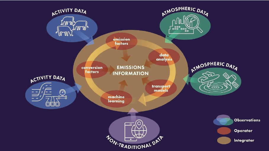
Hybrid approaches derive GHG emissions information through the combination and more complete integration within and between the different approaches described thus far (Figure 2-6). Hybrid approaches are just starting to be developed and there are presently few examples, but many potential directions for further development. For example, a deeper integration of the atmospheric- and activity-based approaches, beyond what is practiced in the current suite of inverse studies, might functionally combine emission processes and atmospheric transport modeling such that atmospheric observations are directly adjusting emission factors or activity data. Another example is an activity-based approach with multiple overlapping core datasets further constrained by atmospheric-based mass balance estimates. Hybrid approaches may also take advantage of a range of new or nontraditional data sources combined with machine learning (ML) techniques that can efficiently analyze large datasets and derive relationships between activity, infrastructure, and GHG emissions in potentially new ways. The hybrid approach classification is less categorically distinct when compared to activity- or atmospheric-based approaches and represents a continuum of simple to more complex efforts aimed at greater integration and combination of the many measurement and modeling efforts to estimate GHG emissions and removals. This section provides an overview of existing and notional examples representing a trajectory toward more integration of existing approaches.
Information Integration Via Data Assimilation
Data assimilation as practiced by numerical weather prediction is a useful model for a more integrated approach to quantifying GHG emissions. In contrast to atmospheric inversions already described, a data assimilation approach could expand the central model from an atmospheric transport model to a dynamical model that simulates GHG emissions and sinks and moves the fluxes through the atmosphere. In this way, the observational constraint moves beyond the prior flux and mixing ratio combination to a wider array of observed quantities, focusing on correcting and estimating the flux model parameter space instead of the fluxes (e.g., Kaminski et al., 2022; Rayner et al., 2005). Elements of activity data (e.g., continuous emission monitors, traffic counters, and gas meter data) in addition to atmospheric concentrations can be directly ingested into a core assimilation model offering degrees of constraint dictated by uncertainty. State estimation-based approaches (e.g., European Centre for Medium-Range Weather Forecasts) can quantify potential biases in activity-based estimates by comparing calculated and observed GHG concentrations, rather than emissions or fluxes (e.g., Weir et al., 2021). State estimation-based approaches are often based on an online meteorological or Earth system model, rather than an offline transport model, and can directly contribute to concentration monitoring as well as large-scale mitigation impact assessment in a more integrated manner (e.g., GHGs and air quality).
Other possibilities might integrate atmospheric-based measurements with other types of measurements not typically included in atmospheric inversions. For example, combining atmospheric measurements (e.g., aircrafts or drones) with novel continuous measurement technologies, especially for methane emissions detection, could help to establish the frequency and duration of emission events at a facility or larger basin level (e.g., Allen et al., 2022; Chen et al., 2022b; Wang et al., 2022b), and the impacts on regional emissions as a whole. Such approaches may hold potential
for the development of empirical-based annualized inventory estimates, especially in the oil and gas sector.
Alternative Data Integration Through Machine Learning
Recent advances in ML—the application of computational algorithms usually applied to large-scale datasets to simulate human learning (Wang et al., 2009)—represent another potential hybrid GHG estimation approach to model complex, nonlinear, and nonparametric relationships between data to achieve potentially more complete and new GHG emissions information. ML algorithms and ML-powered models can take a series of data inputs to train a model to uncover statistical patterns, making predictions on new, “unseen” data (Huntingford et al., 2019; Milojevic-Dupont and Creutzig, 2021). These approaches are now being applied to massive datasets, incorporating multiple data types, and often integrated within emerging digital infrastructures (e.g., blockchains, distributed ledgers; see Box 2-6). While these approaches have the potential to address critical GHG emissions information gaps, including temporal and spatial resolution of existing data, they could undermine transparency needed for credible GHG accounting because ML algorithms are prone to be criticized as a “black box” due to their complexity and often difficulty in interpretation (Castelvecchi, 2016) (see Chapter 3).
To date, ML approaches have been applied in four broad categories related to Earth observation (EO): feature classification (e.g., land use or land cover and land cover change), anomaly, target and change detection, and regression-based methods (e.g., estimating a variable of interest such as GHG emissions from a set of underlying predictor variables) (Salcedo-Sanz et al., 2020). Since ML trains a computer to “learn” and identify relationships with data inputs, ML could improve the performance of traditional data fusion algorithms and approaches (Meng et al., 2020).
An example ML application to GHG emissions estimation is the use of ML-driven predictive models that take advantage of large EO datasets and high-resolution satellites that are capable of measuring land cover and atmospheric conditions. Given these two trends, there is active development of ML algorithms that attempt to estimate GHG emissions at multiple scales (i.e., national and subnational) given known emissions drivers—electricity generation, mobile transport, industry, deforestation, and land-use change (Akhshik et al., 2022; Hamrani et al., 2020; Han et al., 2021; Hsu et al., 2022). Two primary ML-based GHG estimation approaches exist: top-down methods that estimate emissions from socioeconomic and demographic drivers (from Hsu et al., 2022) and bottom-up approaches that characterize infrastructure or activity data rather than the emissions themselves. In the latter application, Climate TRACE has convened a consortium of more than 12 organizations developing ML-based approaches to estimate activity data (e.g., how frequently a power plant is in operation) and GHG emissions (Climate TRACE, n.d.) (see Case Study 4.6).
Numerous research studies are exploring ML-based approaches. Alova et al. (2021), for instance, developed an ML-based model to predict Africa’s electricity generation mix in 2030 using asset-level data on current and planned power plants. Meanwhile, Han et al. (2021) utilized ML to estimate corporate GHG emissions data, incorporating more than 1,000 variables including industry sector classification data, revenue, corporate locations, and ESG data. Niu et al. (2020) applied neural network ML algorithms and random forests—an ML technique used to solve regression and classification problems—to determine 25 socioeconomic characteristics, such as gross domestic product growth rate, population, demographic structure, energy and industrial structure, energy intensity, and environmental policy stringency, and then used these variables to forecast scenarios of China’s future emissions trajectory. While these recent studies provide some potential for ML approaches to address gaps and yield new insights and information for GHG emissions, to what degree they will improve upon existing activity- or atmospheric-based approaches is still uncertain.
More research and development, particularly in exploring the ways artificial intelligence and ML approaches could improve GHG estimation methods, are critical to expanding their application.
Current Status and Uncertainties of Greenhouse Gas Emissions Estimates
Accuracy and uncertainty in GHG emissions estimates vary by type of emission-producing activity, spatial and temporal scale, GHG considered, and the technique used. In addition to the absolute uncertainty, uncertainty associated with a change in emissions over time is also important, particularly for emission reduction targets that are based on trends. Methods of assessing accuracy
and uncertainty include examination of underlying data, emission factors, and approaches (Andres et al., 2014); comparisons of different activity-based emissions estimate products (e.g., Andrew, 2020; Friedlingstein et al., 2022); the inclusion of uncertainty estimates in the calculation for a product (e.g., Asefi-Najafabady et al., 2014; Solazzo et al., 2021); and independent assessment. In this section, we provide a summary of the current state of knowledge for emissions and indicate where activity-based methods are used to quantify uncertainties and in which areas atmospheric-based approaches also contribute.
The most accurate and precise estimates are available for emission-producing activities that have explicit economic value (e.g., energy production). National CO2 emissions from fossil fuel burning are typically well characterized by economic data on fossil fuel trade and production, though there are large uncertainties for many countries. Thus, globally, fossil fuel CO2 emissions are thought to be known with less than ±8 percent 2 sigma uncertainty (Andres et al., 2014) based on an intercomparison of different activity-based products, although many of these products do share input data such as IEA fuel statistics. While uncertainty in national fossil fuel CO2 emissions totals for some nations with excellent data systems may be less than ±5 percent, countries with less well-developed energy data have been uncertainties of ±10 percent or more (Andres et al. 2014; Friedlingstein et al, 2022a; Marland, 2008). Smaller spatial and temporal scales (i.e., subnational, sub-annual) may increase uncertainty because approximation and/or estimation (e.g., proxy data) are often used that may be less directly linked with emissions and vary more across estimation techniques. However, in instances where direct estimation of emissions at smaller scales (e.g., at the point of combustion) is deployed, uncertainty may be lower than when aggregate amounts are downscaled. At 1–100 km resolution (i.e., relevant to cities and U.S. counties) the differences in fossil fuel CO2 emissions among different products can be substantial and estimates vary depending on the approaches (Andres et al., 2016; Fischer et al., 2017; Oda et al., 2019).
Estimates of CO2 emissions from land use and land-use change typically have much larger fractional uncertainties than fossil fuel CO2. Globally, CO2 emissions from land use and land-use change currently have uncertainties of roughly ±75 percent (±0.7 GtC yr−1 in 2020) (Friedlingstein et al., 2022). This estimated uncertainty has undergone large revisions recently using atmospheric-based approaches and may change in the future as different methodologies are compared in more detail (Bastos et al., 2021; Grassi et al., 2021; Petrescu et al., 2020). For individual countries or regions, uncertainties in CO2 emissions from land use and land-use change can be more than ±100 percent (McGlynn et al., 2022).
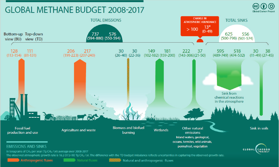
Global total methane emissions have been estimated to ±5 percent by atmospheric-based approaches using measurements of the atmospheric methane growth rate and knowledge of the methane lifetime; however, highly uncertain natural emissions from wetlands, reservoirs, and other sources limit the atmospheric-based constraints on global anthropogenic emissions (Figure 2-7) (Saunois et al., 2020). Using isotopic measurements to isolate fossil fuel-derived methane emissions suggests global emissions of methane from the fossil fuel industry are 50 percent larger than inventory estimates (Hmiel et al., 2020; Schwietzke et al., 2016). The uncertainty of methane emissions from anthropogenic sources was documented in a 2018 report from the National Academies of Sciences, Engineering, and Medicine (NASEM, 2018). Other evidence of underestimated methane emissions from fossil fuel sources comes from atmospheric-based studies showing strong natural gas emissions in urban areas (Saboya et al., 2022; Sargent et al., 2021), areas of gas production (Alvarez et al., 2018), and the presence of super-emitters (Lauvaux et al., 2022) (see Case Study 4.4). Anthropogenic methane emissions from agriculture and waste also have large uncertainties (up to ±70%) (Solazzo et al., 2021) although there have been fewer independent studies to assess their accuracy (e.g., Miller et al., 2019).
For N2O, the largest emission sources are from agriculture and they are known to be highly uncertain (up to ±200%) because they result from the processing of nitrogen fertilizers in soil that can depend on environmental conditions (Solazzo et al., 2021). Atmospheric measurements indicate N2O emissions are underestimated globally (Thompson et al., 2019), although good correspondence has been found between atmospheric data and inventory estimates for some countries (Ganesan et al., 2015).
For the industrially-produced fluorinated gases (i.e., CFCs [chlorofluorocarbons], HCFCs [hydrochlorofluorocarbons], HFCs, PFCs [perfluorocarbons], SF6 [sulfur hexafluoride], and NF3 [nitrogen trifluoride]), their global emissions can be well constrained by atmospheric-based approaches using measurements of the atmospheric growth rate and knowledge of the lifetime for each gas since there are no natural emissions. Atmospheric measurements have revealed unexpected emissions of several fluorinated gases, including CFC-11 (Box 2-7) (Montzka et al., 2018; Rigby et al., 2019), HFC-23 (Stanley et al., 2020), and HCFCs (Vollmer et al., 2021). For the HFCs, most existing inventory estimates do not report uncertainties (Flerlage et al., 2021). Moreover, not all emissions are reported because many countries are non-Annex I Parties to the UNFCCC that are not required to report HFC emissions, although most are now required to report production and consumption (not emissions) as part of the Kigali Amendment to the Montreal Protocol. Emissions from “banks” (stocks of CFCs, HCFCs, and HFCs in existing equipment and foams) are poorly constrained and contribute to emissions uncertainty (UNEP, 2019, 2021b; WMO, 2021). Uncertainties in regional fluorinated gas emissions from atmospheric based studies can range between ±20 percent to ±80 percent, where both underestimates and overestimates have been found for fluorinated gas emissions from individual countries (Flerlage et al., 2021; Manning, 2011).
For tropospheric ozone, GHG precursors (CO, NMVOCs [non-methane volatile organic compounds]), aerosols (BC [black carbon], OC [organic carbon], PM [particulate matter]), and aerosol precursors (SO2 [sulfur dioxide], NOx [nitrogen oxides], NH3 [ammonia]), the global uncertainty is much greater due to their short lifetime. As a result, they are not well mixed in the atmosphere and are subject to large variations in space and time. Since most of these are air pollutants, they are typically monitored by air pollution monitoring networks and satellites.
Tropospheric ozone is not directly emitted, rather emissions of precursors including methane, NMVOCs, CO, and NOx affect the amount of tropospheric ozone in the atmosphere (ozone burden). The uncertainties in global tropospheric ozone burden assessed using atmospheric-based approaches are on the order of 5 to 10 percent (Szopa et al., 2021).
Activity-based uncertainties of anthropogenic emissions of black carbon (BC) typically range from –30 to +120 percent and –40 to +130 percent for organic carbon (Klimont et al., 2017). Large ranges in emissions factors can contribute to higher uncertainties, as in the case of flaring (e.g., Conrad and Johnson, 2017).
Improved accounting of these short-lived pollutants has direct implications for understanding current and future climate impacts in addition to impacts on human health and food productivity. For example, incorrect anthropogenic aerosol emissions over China resulted in flawed model projections (Wang et al., 2021) with important implications for the net anthropogenic aerosol forcing trend (Quaas et al., 2022). Similarly, accounting only for CO2 emissions from aviation without accounting for non-CO2 emissions and contrails could leave significant warming unaddressed and compromise meeting temperature targets (Brasseur and Gupta, 2010; Brazzola et al., 2022; Wuebbles et al., 2007).


