7

Ecosystems

Ecosystems supply the services on which all life depends. Understanding how ecosystems are changing and how these changes influence the Earth system are important for sustaining life on the Earth. Observing and understanding ecosystems and their change is both a major theme in the Decadal Survey (NASEM, 2018) and a key component of a broad range of science and application questions in the report. This chapter describes the geodetic infrastructure required to meet new scientific needs related to ecosystem science. The ecosystems-related science questions which use active remote sensing and thus rely on the geodetic infrastructure are:

E-1. What are the structure, function, and biodiversity of the Earth’s ecosystems, and how and why are they changing in time and space?

E-2. What are the fluxes (of carbon, water, nutrients, and energy)between ecosystems andthe atmosphere, the ocean and the solid Earth, and how and why are they changing?

E-3. What are the fluxes (of carbon, water, nutrients, and energy) within ecosystems, and how and why are they changing?

E-4. How is carbon accounted for through carbon storage, turnover, and accumulated biomass? Have all of the major carbon sinks been quantified and how are they changing in time?

S-4. What processes and interactions determine the rates of landscape change?

The geodetic needs associated with each question appear in the Ecosystems Science and Applications Traceability Matrix (see Appendix A, Table A.5). In this chapter, the discussion of geodetic needs is organized around four themes: vegetation dynamics; lateral transport of carbon, nutrients, soil and water; global soil moisture; and permafrost and changes in the Arctic.

VEGETATION DYNAMICS

Understanding vegetation dynamics, including structure and function, requires a knowledge of the three-dimensional structure of terrestrial and aquatic vegetation over space and time (e.g., Pugh et al., 2019). Previous studies have demonstrated the efficacy of lidar and radar for quantifying forest and aquatic biomass (Liu et al., 2015; Du et al., 2017), characterizing rangeland (Streutker and Glenn, 2006), estimating vegetation height (Hopkinson et al., 2005), monitoring (Rosso et al., 2006), and assessing biodiversity and habitats (Bergen et al., 2009). In addition, optical, lidar, and radar (active and passive) are important for monitoring essential biodiversity variables (Vihervaara et al., 2017; see Box 7.1). Interferometric Synthetic Aperture Radar (InSAR) and Polarimetric SAR Interferometry (Pol-InSAR) are the primary radar techniques used to obtain vegetation structure as well as to understand change over time (Ghasemi et al., 2011; Berninger et al., 2018).

In addition to active radar techniques, passive microwave satellite (using vegetation optical depth) and Global Navigation Satellite System Interferometric Reflectometry (GNSS-IR) data have been found useful for understanding changes in land surface phenology (Jones et al., 2013; Chaparro et al., 2018). GNSS-IR uses ground GNSS receivers to measure the reflection amplitude, which is used for vegetation studies. However,

the utility of GNSS-IR signals for estimating vegetation water content changes (Small et al., 2014) and for studying drought (Small et al., 2018) is an emerging area of study. Amplitude reflections from GNSS Reflectometry (GNSS-R) are sensitive to changes in soil moisture and inundation and thus can be used for mapping wetland ecosystem dynamics (Jensen et al., 2018). While global lidar is not yet available, tropical and temperate forest structure will be measured at roughly 1 km by the Global Ecosystem Dynamic Investigation (GEDI) on the International Space Station (Qi et al., 2019).

Measurements

The vertical accuracy of data from the technologies mentioned previously is a distinguishing characteristic that dictates the horizontal and vertical scales at which vegetation structure and function can be studied (see Figure 7.2). For example, to obtain vertical vegetation structure and derivatives, scientists require lidar (or SAR) with <1 m vertical resolution in forested ecosystems and <0.30 m vertical resolution in dryland ecosystems. For these studies, accuracy and scale depend strongly on land cover and microtopography (e.g., Glenn et al., 2011). For most ecosystems, a 0.1 m or better lidar bare-earth model is needed to derive many of the products necessary for understanding vegetation dynamics. Horizontal precision of lidar is required at roughly 1 m for bare-earth topography for canopy structure use. Annual repeats of airborne lidar surveys are needed, especially in areas with dynamic landscapes.

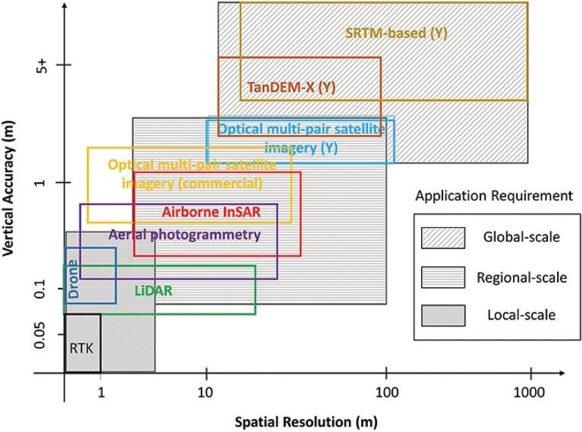
For regional studies that use SAR (L- and P-band), a 10-m global digital elevation model (DEM) is necessary to understand vegetation dynamics. A bare-earth DEM is used as a reference for SAR methods, but is less critical for Pol-InSAR methods. Necessary repeat periods for SAR data range from every 6 days to daily in high latitudes (for freeze-thaw applications, see “Permafrost and Changes in the Arctic” below). SAR data are also needed to augment the coarser sampling of GEDI for forest heights (see Figure 7.3).

Geodetic Needs

The measurements discussed above require maintenance of the current terrestrial reference frame (TRF) for precision positioning with lidar. In remote areas such as Alaska and the Arctic, more base stations (approximately every 30 km without L5 frequency or 50 km with L5 frequency) are needed to develop the 0.1 m lidar bare-earth topography model. L5 frequency is a GNSS frequency with improved signal strength. Tracking L5 in addition to L1 and L2 frequencies provides greater accuracy in these ionospherically active regions.

Determining water vapor from GNSS-derived total column water vapor and additional radio occultation (RO) measurements is needed for SAR correction. Recent simulations indicate that at least 20,000 occultations per day are needed (IROWG, 2017). For example, errors in water vapor will cause errors in biomass estimates. To derive vertical biomass structure using InSAR, the long-wavelength errors need to be reduced by staying within the critical baseline.

For ecosystem studies using GNSS-IR, it is important to configure the ground stations to remove elevation angle masks and to archive the required signal-to-noise ratio (SNR). The low elevation angle GNSS data provide the largest ecosystem footprints. GNSS networks installed by most geoscientists already store SNR data and track low elevation angle signals, and this needs to become standard practice. The GNSS-IR data will need to be augmented with soil moisture sensors distributed across environmental gradients to obtain more comprehensive information on ecosystems and soil moisture. These new products are also useful for calibration and validation of satellite missions.

LATERAL TRANSPORT OF CARBON, NUTRIENTS, SOIL, AND WATER

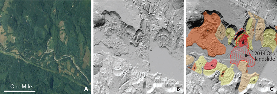
Lateral transport of carbon, nutrients, soil, and water is a key process in the terrestrial carbon cycle. For example, mangroves are highly productive ecosystems that provide carbon storage as well as discharge terrestrial carbon to the ocean (Alongi, 2014). In terrestrial ecosystems, a recent satellite-based study showed that nutrients originating in the Sahara can travel thousands of kilometers and feed the Amazonian forest (Yu et al., 2015). Hillslopes and coastal erosion can transport substantial amounts of carbon (e.g., Naipal et al., 2018; Braun et al., 2019). Landslides, often triggered by weather events, transport rock and alter the Earth’s surface (Hilley et al., 2004). An example is the Oso landslide (see Figure 7.4).

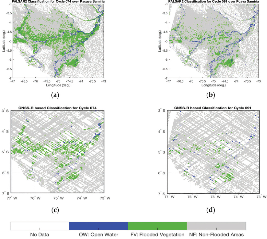
The lateral transport of carbon, nutrients, soil, and water can be quantified with geodetic techniques when the surface displacements are coherent. Particularly relevant are surface displacements associated with landscape change, including subsidence or uplift from volcanic or tectonic processes, and geomorphic (e.g., landslides, channel incision), hydrologic (precipitation, freeze/thaw, and snow accumulation and melt), cryosphere (e.g., ice streams and permafrost thaw), or ecological (e.g., vegetation structure) change. Measuring rates of landscape change and lateral processes, as well as the processes that drive changes, require mm- to m-level vertical and horizontal accuracies, depending on the process being measured (Lambin et al., 2003; Jorgenson and Grosse, 2016). The use of space based reflections (GNSS-R) is emerging as a critical measurement for studying lateral transport from landslides (Carlà et al., 2019) and wetlands (Jensen et al., 2018). For example, GNSS-R was used to understand inundation dynamics of wetlands in the Peruvian Amazon (see Figure 7.5). The variability of wetland extent and inundation plays an important role in ecosystem dynamics and ecosystem services. In addition, wetlands are the largest natural source of methane, contributing roughly 30 percent of global methane emissions (Kirschke et al., 2013), with substantial uncertainty associated with wetland extent (Saunois et al., 2016).

Measurements

A key geophysical observable for understanding landscape processes is the change in bare-earth topography, that is, the change in the Earth’s surface devoid of above-ground biomass. Recent studies have demonstrated the need for high resolution (<0.1 m) bare-earth topographic models for modeling mass transport across landscapes (Passalacqua et al., 2015), and for supporting sustained gravity measurements for assessing changes in water storage across space and time (Pail et al., 2015).

Vertical and horizontal measurements of landscape change depend on whether surface motions are uniform over a relatively broad area (e.g., earthquakes, volcanic inflation, and large landslides) or are highly localized (e.g., displacement of soil, rock, or vegetation on the surface). For broad areas where the surface remains coherent, GNSS-IR and repeat-pass InSAR are optimal techniques for measuring mm changes (see Chapter 5). However, InSAR cannot measure landscape change where the rock or soil is locally deformed because the reference and repeat images are decorrelated. Measuring this surface change is best done using repeat lidar measurements from spacecraft or aircraft.

Numerous studies have shown that repeat topographic surveys with spatial resolution of 1 m and vertical precision of 0.1 m can resolve most of the important landscape changes. The best global space-based topography grids are from the TanDEM-X mission, and they have a spatial resolution of ~10 m and measure the top of the canopy, rather than bare earth. The Ice, Cloud, and land Elevation Satellite (ICESat-2) laser altimeter would take more than 600 years to map the Earth at 1 m spatial resolution.¹ Development of a multibeam lidar (~1,000 beams) would reduce the mapping time to about 4 years, which is still inadequate to resolve many landscape processes. Given these constraints, the best way to obtain the necessary time series may be to acquire a global, baseline high-resolution topographic data set and revisit select areas using an airborne lidar having a 1 m resolution and 0.1 m vertical precision.

In coastal areas, the vertical measurement needs to have an accuracy of 0.1 m or better with respect to the TRF to provide a connection with absolute sea level. This accuracy requirement also covers coastal areas where permafrost soil has retreated. Achieving this accuracy using aircraft lidar will require deployment of several GNSS base stations within 30–50 km of the survey area, depending on whether the aircraft is tracking multi-GNSS.

Spatial and temporal requirements for lateral transport from a water budget perspective include improved measurements of evapotranspiration, snow, and water storage (Lettenmaier et al., 2015). Finer temporal and spatial scale gravity measurements are needed to capture basin geometry as well as to capture basins at high latitudes. Accurate fine-scale DEMs (<10 m) and GNSS every 100 km (or <50 km without Gravity Recovery Climate Experiment gravity measurements) are needed to help calculate better estimates of water storage change, especially in small- to mid-size basins, and thus to track lateral carbon exchanges (e.g., Knappe et al., 2018). Similarly, surface water measurements need to capture high temporal dynamics associated with processes such as flooding and wetland inundation. For these dynamic processes, Surface Water Ocean Topography measurements of 250 m × 250 m-sized water bodies (the science objective) can be spatially complemented with measurements from ICESat-2, GNSS-R, GNSS-IR, and the upcoming NISAR mission. Multiple pairs of satellites or reflections from closely-spaced GNSS stations are required to fully capture spatial and temporal dynamics. Estimates of lateral relocation of sediment, carbon, and nutrients from storm surges and other coastal processes could be improved by using GNSS-IR to measure water levels (Larson et al., 2017).

Geodetic Needs

Lateral transport studies require maintenance of the current geodetic infrastructure. The geodetic needs for both airborne lidar and GNSS are the same as for vegetation dynamics. Collocating GNSS and tide gauges at coastal sites, installing additional geodetic monuments, and using GNSS-IR to measure tides will support measurements of subsidence and coastal erosion for carbon storage changes. The geodetic needs for

___________________

¹ Mapping the circumference of the Earth in meters requires 40,000,000 orbits. There are 14 orbits per day, so that is 7,600 years. ICESat-2 has 6 beams and there are ascending and descending tracks, so divide by 12 for 638 years.

InSAR are also similar to those discussed for vegetation dynamics, with the addition of daily observations in high latitudes (for freeze-thaw dynamics). The InSAR measurements of coherent surface motion will require orbits with precision of 20–40 mm across-track and 40–70 mm along-track, and additional RO measurements and total column water vapor from GNSS for water vapor determination. The geodetic needs for total and surface water storage require an increased number of closely-spaced GNSS stations (100 km or less).

GLOBAL SOIL MOISTURE

Soil moisture is an essential climate variable that modulates vegetation activity (Ali et al., 2015; Karthikeyan et al., 2017). Measurements of soil moisture are necessary to understand ecosystem function and critical zone processes, and they can be made using passive and active microwave. The radiometer on the Soil Moisture Active Passive (SMAP) mission enables global soil moisture measurements to be down-scaled (Abbaszadeh et al., 2019) with up to 4 percent volumetric error in soil moisture. Recently, GNSS-IR signals have been used to estimate soil moisture (Chew et al., 2015). On space platforms, Carreno-Luengo et al. (2018) used CYGNSS, GNSS-R, and SMAP microwave radiometry brightness temperature to estimate soil moisture and distinguish land cover types across the globe.

Measurements

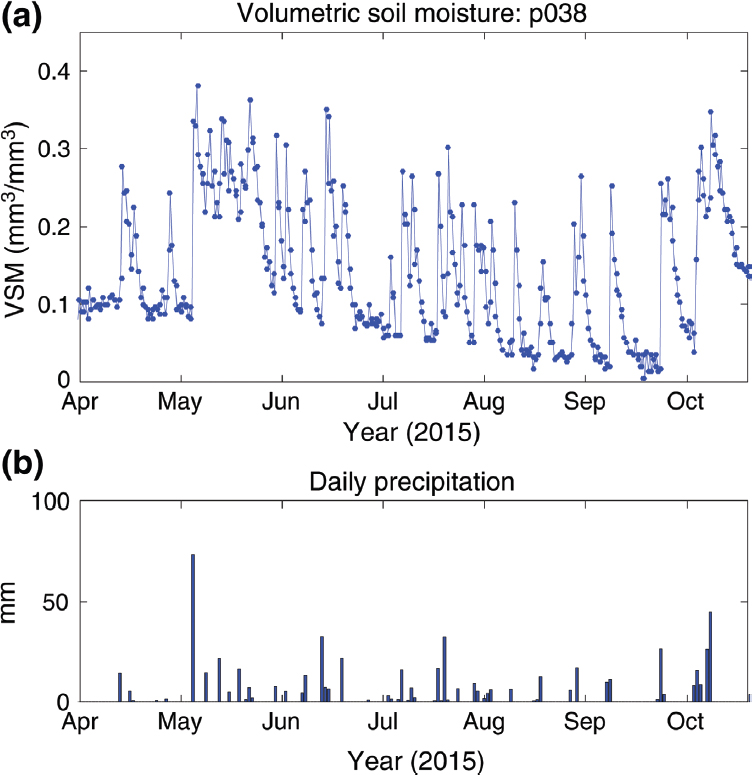
The footprint of each GNSS-IR soil moisture instrument is ~1,000 m². Thus, GNSS-IR is essentially a point measurement, similar to measurements from other continental-scale soil moisture networks, such as the U.S. Climate Reference Network. Nearly all GNSS-based studies of soil moisture have been made using instruments deployed for other purposes. For example, GNSS data from the Plate Boundary Observatory (PBO) were used in the PBO H2O project to create water cycle products (Larson, 2016). Because it met the 4 percent volumetric error accuracy requirement of the SMAP and Soil Moisture Ocean Salinity missions (Small et al., 2016), data from the PBO H2O project were also used for satellite validation (Al-Yaari et al., 2017).

A benefit of PBO H2O was that the GNSS sites were located in more diverse land cover than traditional soil moisture satellite validation sites, which are concentrated in agricultural areas. PBO H2O produced a 7-year record of volumetric soil moisture measurements at more than 125 GNSS sites in the western United States (Larson, 2016). An example of variations in soil moisture and its relationship to precipitation from spring to fall 2015 is shown in Figure 7.6. This project took advantage of the high-quality instrumentation and the coordinated archiving system used by the PBO project, which are not always available from other GNSS networks.

Geodetic Needs

Geodetic needs for global soil moisture measurements are similar to those described above for SAR and GNSS (see the section “Lateral Transport of Carbon, Nutrients, Soil, and Water”). SAR requires the current geodetic infrastructure to be able to precisely geolocate with GNSS/Galileo. GNSS-IR requires access to the raw GNSS observation files, SNR archive, and elimination of elevation angle masks. Current positioning initiatives indicate that more than 15,000 such sites are available on a daily basis worldwide. However, a global effort is currently limited by the lack of standardized community software for soil moisture retrievals. An increase in the number of GNSS sites in vegetated areas and in a range of biomes (e.g., savannahs and grasslands) are needed. The number of GNSS sites could be potentially increased by coordinating with the geological hazards community.

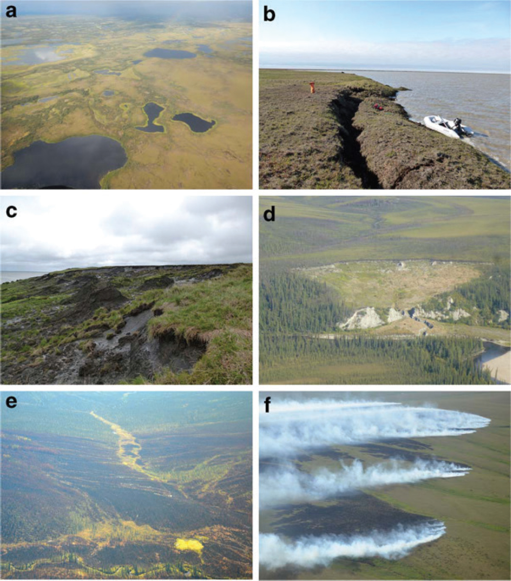
PERMAFROST AND CHANGES IN THE ARCTIC

The geodetic infrastructure plays an important role in understanding a wide variety of processes that operate at high latitudes (see Figure 7.7). A number of different remote sensing observations can be used to understand Arctic processes. For example, satellite gravity is used to measure rock-, soil-, water-, and ice-mass change in high latitudes (Talpe et al., 2017). Lidar and InSAR have been used to track subsidence in the Arctic (Stettner et al., 2017; Whitley et al., 2018). Understanding permafrost dynamics is essential for

understanding carbon dynamics in the Arctic, including the vegetation growth period and soil respiration (Bloom et al., 2016; Nitze et al., 2018). Monitoring temperature transitions when large surges of melt water occur is important for Arctic marine communities (Frainer et al., 2017). In addition to gravity and InSAR, L-band radar backscatter is used to study freeze/thaw (Du et al., 2015); P-band is better for ice penetration (Gusmeroli et al., 2013). L-band and C-band coherence maps from NISAR and Sentinel-1, respectively, will be useful for studies of permafrost and freeze/thaw dynamics, such as noted in Rowland (2010). Compared with InSAR, GNSS-R and GNSS-IR offer enhanced temporal (daily) sensitivity for permafrost studies. The use of ground-based GNSS-IR for this application has been demonstrated for a site in Barrow, Alaska (Liu and Larson, 2018).

Measurements

SAR measurements with at least a 30 m spatial resolution are ideal, because of heterogeneity in the microclimate of the Arctic. Daily measurements are necessary to capture the temporal dynamics. Measuring finer-scale terrain deformation (e.g., ~10 mm-scale variations) using InSAR and airborne lidar is important for understanding some of the variability in the freeze-thaw zones. Repeat lidar surveys with precise relocation over time are necessary to capture permafrost thaw and the resulting mobilization of materials (Rowland, 2010). High-resolution DEMs are needed for vertical resolutions of frozen ground (Westermann et al., 2015). The timing of these measurements is critical because the transition from winter to spring to summer is when most of the dynamics can be accounted for. GNSS-IR requirements are the same as for soil moisture. Recent

InSAR measurements of the freeze-thaw cycles in Tibet require relative orbital accuracies of better than 20–40 mm to recover the 10 mm annual signals (Daout et al., 2017).

Geodetic Needs

Airborne lidar, InSAR, and GNSS-IR measurements are needed for tracking permafrost and changes in the Arctic. The geodetic infrastructure requirements

to support these measurements are the same as those for lateral transport of carbon, nutrients, soil, and water, and vegetation dynamics.

SUMMARY

Maintaining the current TRF is important for ecosystem science. Many measurements in ecosystem science require that the current precision of orbit determination be maintained. The application of GNSS to ecosystem science is emerging, and so the SNR from GNSS should continue to be archived. Sustained gravity measurements are also a priority.

New geodetic needs to help answer the ecosystem science questions in the Decadal Survey include increasing the number of GNSS stations across environmental gradients and placing these stations at locations with tide gauges and soil moisture sensors. These stations should also complement the scale at which gravity measurements are made (e.g., more stations are needed if gravity observations continue to be relatively coarse). In addition, many more RO measurements are needed to support water vapor observations. Land and vegetation topography at 1 m spatial and 0.1 m vertical resolution are needed, both weekly in areas dominated by change, and yearly for most other areas. Finally, cyberinfrastructure, analytical software, and tools, as well as the training to utilize them, need to be made widely accessible to the community, especially to early-career scientists. For example, while lidar and InSAR processing have become more user friendly in the past decade, training and processing software for GNSS reflections are not widely available. Additional support is needed to combine disparate data types (e.g., GNSS, InSAR, PolSAR, and lidar) to augment data gaps. Finally, cyberinfrastructure that allows easy access to pull or push data for processing (e.g., through application programming interfaces) is needed.

The following summarizes needs for maintaining or enhancing the geodetic infrastructure, and related improvements to enhance scientific returns.

Maintenance of the Geodetic Infrastructure

• Maintain the current TRF.
• Maintain orbit determination, with 10–20 mm orbit accuracy, 40–70 mm along-track accuracy, and mm/yr orbit stability.
• Sustained gravity measurements for an accurate geocenter.

Enhancements to the Geodetic Infrastructure

• Additional base stations in remote areas (every 30 km without L5 frequency or 50 km with L5), and more GNSS frequencies (e.g., L5 frequency and the receivers to support additional frequencies).
• Training and cyberinfrastructure to support adoption of above technologies.

Related Improvements to the Geodetic Infrastructure to Enhance Scientific Returns

• Additional GNSS stations (or in situ GNSS-IR) co-located with soil moisture sensors in diverse ecosystems and with tide gauges along coastlines in northern latitudes.
• Gravity every 100 km and GNSS every 50 km. GNSS needs include a regional network in northern latitudes (e.g., Alaska, which has synergies with tectonics applications), and increased temporal resolution (weekly to every 10 days) for monitoring water storage fluxes.
• Increased number of RO measurements and GNSS-derived total column water vapor for SAR and InSAR.

REFERENCES

Berninger, A., S. Lohberger, M. Stängel, and F. Siegert. 2018. SAR-based estimation of above-ground biomass and its changes in tropical forests of Kalimantan using L- and C-Band. Remote Sensing 10(6):831.

Bloom, A.A., J.F. Exbrayat, I.R. van der Velde, L. Feng, and M. Williams. 2016. The decadal state of the terrestrial carbon cycle: Global retrievals of terrestrial carbon allocation, pools, and residence times. Proceedings of the National Academy of Sciences 113(5):1285-1290.

Braun, K.N., E.J. Theuerkauf, A.L. Masterson, B.B. Curry, and D.E. Horton. 2019. Modeling organic carbon loss from a rapidly eroding freshwater coastal wetland. Scientific Reports 9(1):4204.

Carlà, T., V. Tofani, L. Lombardi, F. Raspini, S. Bianchini, D. Bertolo, P. Thuegaz, and N. Casagli. 2019. Combination of GNSS, satellite InSAR, and GBInSAR remote sensing monitoring to improve the understanding of a large landslide in high alpine environment. Geomorphology 335:62-75.

Carreno-Luengo, H., G. Luzi, and M. Crosetto. 2018. Sensitivity of CyGNSS bistatic reflectivity and SMAP microwave radiometry brightness temperature to geophysical parameters over land surfaces. IEEE Journal of Selected Topics in Applied Earth Observations and Remote Sensing 99:1-16.

Chaparro, D., M. Piles, M. Vall-Llossera, A. Camps, A.G. Konings, D. Entekhabi, and T. Jagdhuber. 2018. L-Band vegetation optical depth for crop phenology monitoring and crop yield assessment. In IGARSS 2018. IEEE International Geoscience and Remote Sensing Symposium 8225-8227.

Chew, C.C., E.E. Small, and K.M. Larson. 2015. An algorithm for soil moisture estimation using GNSS-interferometric reflectometry for bare and vegetated soil. GPS Solutions 20(3):525-537.

Daout, S., M.-P. Doin, G. Peltzer, A. Socquet, and C. Lasserre. 2017. Large-scale InSAR monitoring of permafrost freeze-thaw cycles on the Tibetan Plateau. Geophysical Research Letters 44:901-909.

Du, J., J.S. Kimball, M. Azarderakhsh, R.S. Dunbar, M. Moghaddam, and K.C. McDonald. 2015. Classification of Alaska spring thaw characteristics using satellite L-band radar remote sensing. IEEE Transactions on Geoscience and Remote Sensing 53(1):542-556.

Du, W., Z. Li, Z. Zhang, Q. Jin, X. Chen, and S. Jiang. 2017. Composition and biomass of aquatic vegetation in the Poyang Lake, China. Scientifica 2017:8742480.

Frainer, A., R. Primicerio, S. Kortsch, M. Aune, A.V. Dolgov, M. Fossheim, and M.M. Aschan. 2017. Climate-driven changes in functional biogeography of Arctic marine fish communities. Proceedings of the National Academy of Sciences of the United States of America 114(46):12202-12207.

Ghasemi, N., M.R. Sahebi, and A. Mohammadzadeh. 2011. A review on biomass estimation methods using synthetic aperture radar data. International Journal of Geomatics and Geosciences 1:776-788.

Glenn, N.F., L.P. Spaete, T.T. Sankey, D.R. Derryberry, S.P. Hardegree, and J.J. Mitchell. 2011. Errors in lidar-derived shrub height and crown area on sloped terrain. Journal of Arid Environments 75(4):377-382.

Gusmeroli, A., A. Arendt, D. Atwood, B. Kampes, M. Sanford, and J.C. Young. 2013. Variable penetration depth of interferometric synthetic aperture radar signals on Alaska glaciers: A cold surface layer hypothesis. Annals of Glaciology 54(64):218-223.

Haugerud, R.A. 2014. Preliminary Interpretation of Pre-2014 Landslide Deposits in the Vicinity of Oso, Washington. U.S. Geological Survey Open-File Report 2014–1065. http://pubs.usgs.gov/of/2014/1065/pdf/ofr2014-1065.pdf.

Hilley, G.E., R. Bürgmann, A. Ferrietti, F. Novali, and F. Rocca. 2004. Dynamics of slow-moving landslides from permanent scatterer analysis. Science 304:1952-1955.

Hopkinson, C., L.E. Chasmer, G. Sass, I.F. Creed, M. Sitar, W. Kalbfleisch, and P. Treitz. 2005. Vegetation class dependent errors in lidar ground elevation and canopy height estimates in a boreal wetland environment. Canadian Journal of Remote Sensing 31(2):191-206.

IROWG (International Radio Occultation Working Group). 2017. Summary of the Fifth International Radio Occultation Workshop, September 2016. http://www.wmo.int/pages/prog/sat/meetings/documents/IPET-SUP-3_INF_02-01_IROWG5-Minutes-Summary-Feb16-2017VApr2017.pdf.

Jensen, K., K. McDonald, E. Podest, N. Rodriguez-Alvarez, V. Horna, and N. Steiner. 2018. Assessing L-Band GNSS-reflectometry and imaging radar for detecting sub-canopy inundation dynamics in a tropical wetlands complex. Remote Sensing 10(9):1431.

Jones, M.O., J.S. Kimball, E.E. Small, and K.M. Larson. 2013. Comparing land surface phenology derived from satellite and GNSS network microwave remote sensing. International Journal of Biometeorology 58(6):1305-1315.

Jorgenson, M.T., and G. Grosse. 2016. Remote sensing of landscape change in permafrost regions. Permafrost and Periglacial Processes 27(4):324-338.

Karthikeyan, L., M. Pan, N. Wanders, D.N. Kumar, and E.F. Wood. 2017. Four decades of microwave satellite soil moisture observations: Part 1. A review of retrieval algorithms. Advances in Water Resources 109:106-120.

Kirschke, S., P. Bousquet, P. Ciais, M. Saunois, J.G. Canadell, E.J. Dlugokencky, P. Bergamaschi, D. Bergmann, D.R. Blake, L. Bruhwiler, P. Cameron-Smith, S. Castaldi, F. Chevallier, L. Feng, A. Fraser, M. Heimann, E.L. Hodson, S. Houweling, B. Josse, P.J. Fraser, P.B. Krummel, J.-F. Lamarque, R.L. Langenfelds, C. Le Quéré, V. Naik, S. O’Doherty, P.I. Palmer, I. Pison, D. Plummer, B. Poulter, R.G. Prinn, M. Rigby, B. Ringeval, M. Santini, M. Schmidt, D.T. Shindell, I.J. Simpson, R. Spahni, L.P. Steele, S.A. Strode, K. Sudo, S. Szopa, G.R. van der Werf, A. Voulgarakis, M. van Weele, R.F. Weiss, J.E. Williams, and G. Zeng. 2013. Three decades of global methane sources and sinks. Nature Geoscience 6:813-823.

Knappe, E., R. Bendick, H.R. Martens, D.F. Argus, and W.P. Gardner. 2018. Downscaling vertical GNSS observations to derive watershed-scale hydrologic loading in the Northern Rockies. Water Resources Research 55(1):391-401.

Lambin, E.F., H.J. Geist, and E. Lepers. 2003. Dynamics of land-use and land-cover change in tropical regions. Annual Review of Environment and Resources 28(1):205-241.

Larson, K.M. 2016. GNSS interferometric reflectometry: Applications to surface soil moisture, snow depth, and vegetation water content in the Western United States. WIREs Water 3:775-787.

Larson, K.M., R. Ray, and S.P. Williams. 2017. A ten-year comparison of water levels measured with a geodetic GNSS receiver versus a conventional tide gauge. Journal of Atmospheric and Oceanic Technology 34(2):295-307.

Lettenmaier, D.P., D. Alsdorf, J. Dozier, G.J. Huffman, M. Pan, and E.F. Wood. 2015. Inroads of remote sensing into hydrologic science during the WRR era. Water Resources Research 51(9):7309-7342.

Liu, L., and K.M. Larson. 2018. Decadal changes of surface elevation over permafrost area estimated using reflected GNSS signals. The Cryosphere 12:477-489.

Liu, Y.Y., A.I.J.M. van Dijk, R.A.M. de Jeu, J.G. Canadell, M.F. McCabe, J.P. Evans, and G. Wang. 2015. Recent reversal in loss of global terrestrial biomass. Nature Climate Change 5(5):470-474.

Naipal, V., P. Ciais, Y. Wang, R. Lauerwald, B. Guenet, and K. Van Oost. 2018. Global soil organic carbon removal by water erosion under climate change and land use change during AD 1850–2005. Biogeosciences 15(14):4459-4480.

NASEM (National Academies of Sciences, Engineering, and Medicine). 2018. Thriving on Our Changing Planet: A Decadal Strategy for Earth Observation from Space. Washington, DC: The National Academies Press.

Nitze, I., G. Grosse, B.M. Jones, V.E. Romanovsky, and J. Boike. 2018. Remote sensing quantifies widespread abundance of permafrost region disturbances across the Arctic and Subarctic. Nature Communications 9(1):5423.

Pail, R., R. Bingham, C. Braitenberg, H. Dobslaw, A. Eicker, A. Güntner, M. Horwath, E. Ivins, L. Longuevergne, I. Panet, and B. Wouters. 2015. Science and user needs for observing global mass transport to understand global change and to benefit society. Surveys in Geophysics 36(6):743-772.

Passalacqua, P., P. Belmont, D.M. Staley, J.D. Simley, J.R. Arrowsmith, C.A. Bode, C. Crosby, S.B. DeLong, N.F. Glenn, S.A. Kelly, and D. Lague. 2015. Analyzing high resolution topography for advancing the understanding of mass and energy transfer through landscapes: A review. Earth-Science Reviews 148:174-193.

Pugh, T.A.M., M. Lindeskog, B. Smith, B. Poulter, A. Arneth, V. Haverd, and L. Calle. 2019. Role of forest regrowth in global carbon sink dynamics. Proceedings of the National Academy of Sciences of the United States of America 116(10):4382-4387.

Qi, W., S. Saarela, J. Armston, G. Ståhl, and R. Dubayah. 2019. Forest biomass estimation over three distinct forest types using TanDEM-X InSAR data and simulated GEDI lidar data. Remote Sensing of Environment 232:111283.

Quegan, S., T. Le Toan, J. Chave, J. Dall, J.F. Exbrayat, D.H.T. Minh, M. Lomas, M.M. D’Alessandro, P. Paillou, K. Papathanassiou, and F. Rocca. 2019. The European Space Agency BIOMASS mission: Measuring forest above-ground biomass from space. Remote Sensing of Environment 227:44-60.

Rodriguez-Alvarez, N., E. Podest, K. Jensen, and K.C. McDonald. 2019. Classifying inundation in a tropical wetlands complex with GNSS-R. Remote Sensing 11(9):1053.

Rosso, P.H., S.L. Ustin, and A. Hastings. 2006. Use of lidar to study changes associated with Spartina invasion in San Francisco Bay marshes. Remote Sensing of Environment 100(3):295-306.

Rowland, J.C., C.E. Jones, G. Altmann, R. Bryan, B.T. Crosby, G.L. Geernaert, L.D. Hinzman, D.L. Kane, D.M. Lawrence, A. Mancino, P. Marsh, J.P. McNamara, V.E. Romanovsky, H. Toniolo, B.J. Travis, E. Trochim, and C.J. Wilson. 2010. Arctic landscapes in transition: Responses to thawing permafrost. Eos, Transactions, American Geophysical Union 91(26):229-236.

Saunois, M., P. Bousquet, B. Poulter, and 78 coauthors. 2016. The global methane budget 2000-2012. Earth System Science Data 8:697-751.

Schumann, G.J.P., and P.D. Bates. 2018. The need for a high-accuracy, open access global DEM. Frontiers in Earth Science. https://doi.org/10.3389/feart.2018.00225.

Small, E.E., K.M. Larson, and W. Smith. 2014. Normalized Microwave Reflection Index, II: Validation of vegetation water content estimates at Montana grasslands. IEEE Journal of Selected Topics in Applied Earth Observations and Remote Sensing 7(5):1512-1521.

Small, E.E., K.M. Larson, C.C. Chew, J. Dong, and T.E. Oschner. 2016. Validation of GNSS-IR soil moisture retrievals: Comparison of algorithms with different algorithms to remove vegetation effects. IEEE Journal of Selected Topics in Applied Earth Observations and Remote Sensing 9(10):4759-4770.

Small, E.E., C.J. Roesler, and K.M. Larson. 2018. Vegetation response to the 2012-2014 California drought from GNSS and optical measurements, 2018. Remote Sensing 10(4):630.

Stettner, S., A. Beamish, A. Bartsch, B. Heim, G. Grosse, A. Roth, and H. Lantuit. 2017. Monitoring inter-and intra-seasonal dynamics of rapidly degrading ice-rich permafrost riverbanks in the Lena Delta with TerraSAR-X time series. Remote Sensing 10(1):51.

Streutker, D., and N. Glenn. 2006. Lidar measurement of sagebrush steppe vegetation heights. Remote Sensing of Environment 102:135-145.

Talpe, M.J., R.S. Nerem, E. Forootan, M. Schmidt, F.G. Lemoine, E.M. Enderlin, and F.W. Landerer. 2017. Ice mass change in Greenland and Antarctica between 1993 and 2013 from satellite gravity measurements. Journal of Geodesy 91(11):1283-1298.

Vihervaara, P., A.P. Auvinen, L. Mononen, M. Törmä, P. Ahlroth, S. Anttila, K. Böttcher, M. Forsius, J. Heino, J. Heliölä, and M. Koskelainen. 2017. How essential biodiversity variables and remote sensing can help national biodiversity monitoring. Global Ecology and Conservation 10:43-59.

Westermann, S., C.R. Duguay, G. Grosse, and A. Kaab. 2015. Remote sensing of permafrost and frozen ground. In Remote Sensing of the Cryosphere, M. Tedesco, ed. https://doi.org/10.1002/9781118368909.

Whitley, A.M., V.G. Frost, T.M. Jorgenson, J.M. Macander, V.C. Maio, and G.S. Winder. 2018. Assessment of lidar and spectral techniques for high-resolution mapping of sporadic permafrost on the Yukon-Kuskokwim Delta, Alaska. Remote Sensing 10(2):258.

Yu, H., M. Chin, T. Yuan, H. Bian, L.A. Remer, J.M. Prospero, A. Omar, D. Winker, Y. Yang, Y. Zhang, Z. Zhang, and C. Zhao. 2015. The fertilizing role of African dust in the Amazon rainforest: A first multiyear assessment based on data from Cloud-Aerosol Lidar and Infrared Pathfinder Satellite Observations. Geophysical Research Letters 42(6):1984-1991.

REFERENCES

Abbaszadeh, P., H. Moradkhani, and X. Zhan, 2019. Downscaling SMAP radiometer soil moisture over the CONUS using an ensemble learning method. Water Resources Research 55(1):324-344.
Al-Yaari, A., J.P. Wigneron, Y. Kerr, N. Rodriguez-Fernandez, P.E. O’Neill, T.J. Jackson, G. De Lannoy, A. Al Bitar, A Mialon, P. Richaume, J.P. Walker, A. Mahmoodi, and S. Yueh. 2017. Evaluating soil moisture retrievals from ESA’s SMOS and NASA’s SMAP brightness temperature datasets. Remote Sensing of Environment 193:257-273.
Ali, I., F. Greifeneder, J. Stamenkovic, M. Neumann, and C. Notarnicola. 2015. Review of machine learning approaches for biomass and soil moisture retrievals from remote sensing data. Remote Sensing 7(12):16398-16421.
Alongi, D.M. 2014. Carbon cycling and storage in mangrove forests. Annual Review of Marine Science 6:195-219.
Bergen, K.M., S.J. Goetz, R.O. Dubayah, G.M. Henebry, C.T. Hunsaker, M.L. Imhoff, R.F. Nelson, G.G. Parker, and V.C. Radeloff. 2009. Remote sensing of vegetation 3-D structure for biodiversity and habitat: Review and implications for lidar and radar spaceborne missions. Journal of Geophysical Research: Biogeosciences 114(G2):G00E06.