
6
Standard and Evolving Subsurface Characterization
Prior chapters introduced types of steel, the earth materials in which steel is placed, and the corrosion processes that affect underground steel infrastructure. Chapter 4 established that the propensity for and rate of steel corrosion are more greatly influenced by the characteristics of the subsurface environment rather than the composition of any of the steels that are currently economical, practical, and in common use for buried-steel applications. Therefore, a comprehensive understanding of the subsurface is essential to model accurately the corrosion of buried steel. From a corrosion risk perspective, subsurface characterization includes identifying components of the subsurface that may contribute to the corrosivity of the environment. Many test methods used in corrosion investigations were adapted from methods developed for application in the field of agronomy. While tests completed in the laboratory setting yield precise measurements at a single point in space and time, the results may not necessarily represent field conditions because of changes in the biogeochemistry during transport and sample preparation. These tests are referred to in this report as “screening tests.” In contrast, in situ field analyses are typically completed with field parameters relatively intact but often are limited in their resolution given the heterogeneity of the subsurface. Given the difficulties characterizing a spatially and temporally variable subsurface, characterization techniques—both laboratory and field—at different scales are often combined. These analyses are used to assess the magnitude of subsurface corrosivity, estimate corrosion rates, and determine appropriate corrosion protection measures. However, corrosion rate estimates often do not include propagated error, nor do they reflect possible temporal variability in conditions, nor on how temporal variability will be affected by global climate change (e.g., changing temperatures, rainfall and soil-moisture conditions, changing soil-ionic content as a result of sea level rise [see, e.g., Zhang et al., 2022]). Additionally, the lack of field data from long-term and well-controlled experiments (see Chapter 2) poses a significant challenge for the assessment of the efficacy and uncertainty of predictive models that integrate many of these subsurface characteristics (see Chapter 8). The committee finds it is unable to draw conclusions regarding the efficacy of current practices.
This chapter explores current field and laboratory subsurface characterization techniques that inform the prediction, assessment, and modeling of soil corrosivity and corrosion rates of steel structures in the subsurface, as well as how those techniques are evolving. Although there are numerous techniques used to characterize the subsurface, this chapter focuses on those associated with understanding corrosivity of the subsurface environments and the corrosion rates of steel placed in them. The chapter focuses on understanding corrosivity and corrosion rates of steel buried in soils because steel is less commonly in direct contact with in situ rock (steel piles may be
driven through soil to sit on top of in situ rock, and mechanical reinforcing rock bolts may be rarely or temporarily inserted into rock; see Table 2.1).
The chapter first describes the subsurface characterization that occurs before and during installation, then discusses subsurface characterization that occurs during operation and after failure in a forensic setting, and finally describes some emerging characterization methods. Note that there are often several methods that seem to be similar or seem to provide similar results. This is a result of different methodologies being developed for different industries or by different equipment manufacturers who have developed their own patents. The existence of these multiple methodologies that target similar parameters may be interpreted to signify that no single methodology has yet been developed that provides all the information needed, and that each of the methods has distinct advantages and disadvantages. The committee does not attempt to rank or recommend the use of one methodology over another but describes these methods with the understanding that there are uncertainties inherent in the use of any of them. Box 6.1 provides a list of common terms used in this chapter and the remainder of this report.
STANDARD PRACTICE BEFORE AND DURING INSTALLATION
The evaluation of soil corrosivity often depends on standards of practice in a local geographic region. If a given locality has not been considered historically to be corrosive, then there may be only modest in situ or laboratory testing to determine corrosivity. On the other hand, if a given locality is known to have properties conducive to corrosion, such as high concentrations of chloride, or if a locality has not previously been extensively studied, then explicit in situ and laboratory testing from samples may be performed. Most soil corrosivity testing is conducted traditionally through laboratory testing of bulk samples collected by disturbed sampling at the site and not from in situ field testing.
At the start of any investigation, whether for gathering general geotechnical property information or specifically to characterize corrosivity of a site, the geotechnical engineer will search for historical information from, for example, existing geological maps from the U.S. Geological Survey (USGS) or other sources, and from boring and monitoring well logs proximate to the site that may have been cataloged by local building authorities or other project owners. Local and city building authorities may have records (often publicly available online). Such historical information can guide the need for additional study. Good practice for geotechnical engineers is to also consider the possible presence of stray currents (see Box 6.2).
If available information is not sufficient to inform decision making related to design, corrosion control, or operation and maintenance, then the engineer needs to develop a field and laboratory investigation to study soil corrosivity. Selected laboratory testing to characterize corrosivity will be conducted on bulk soil samples collected during the geotechnical investigation to establish design parameters. The amount and type of corrosivity testing typically is based on a balance of anticipated variation in overall site conditions and costs. In practice, it is rare to conduct laboratory corrosivity testing on bulk samples from every boring location and at every depth as might typically be done to characterize geotechnical and physical properties for design. As a result, heterogeneity in those properties that might be conducive to corrosivity may not be captured.
In some cases, especially for large geo-civil infrastructure projects or oil and gas pipelines, in situ field corrosivity testing may also be conducted to complement laboratory testing of field samples. The principal reason is that steel may penetrate multiple soil strata, and the lateral character of the soil conditions may also vary significantly over the project site. The more common field methods currently in use to assess corrosivity include electromagnetic measurements and electrical resistivity. These methods are discussed later in this chapter.
Laboratory Methods
Laboratory methods provide quantitative measurements of soil and groundwater characteristics and properties under controlled and repeatable testing conditions. These tests are designed to measure a single variable (e.g., pH) for a sample taken at a single point in time and in space; consequently, the results are inherently limited in their spatial and temporal scale. Laboratory methods can be divided into laboratory tests, screening tests, or index tests (which do not quantify material properties or characteristics directly) (see Box 6.1). Procedures for measuring soil electrochemical properties are described in a variety of standards and recommendations from the American Association of State Highway and Transportation Officials (AASHTO), ASTM International, the American Water Works Association (AWWA), the American Public Health Association, the Soil Science Society of America, the USGS, the U.S. Environmental Protection Agency, and the Natural Resources Conservation Soil Survey. Different standards for laboratory methods serve specific industries and different locales, and the standards often apply the same general techniques but may differ in recommendations for sample preparations or treatments. Some state departments of transportation have developed their own testing procedures (e.g., California, Nevada, North Carolina, Pennsylvania, and Texas) because of unique construction practices, such as the use of coarser materials for fill due to local availability. The choice of applicable standards is based on the infrastructure type and location.
For example, practices related to a transportation asset such as a mechanically stabilized earth (MSE) wall will generally follow AASHTO standards unless the MSE wall is in a jurisdiction with its own standard. Agencies that build infrastructure without their own governing standards (e.g., the U.S. Bureau of Reclamation) often use international guidelines such as those written by ASTM International.
Many tests performed to identify soils that contribute to corrosion are consensus standard tests, which balance factors such as test complexity and analytical precision with cost and limited accessibility to sophisticated laboratory equipment. In Tables 6.1 and 6.2, both ASTM and AASHTO standards are cited when they are equivalent (e.g., AASHTO T 265-15, 2019 and ASTM D2216-19, 2019 for moisture content). In other cases, more than one test standard exists for measurement of a given property, but there are differences in terms of sample treatments and preparations. For example, resistivity and pH can be measured via AASHTO T 288-12 (2016) and AASHTO
TABLE 6.1 Example Laboratory Test Methods Consistently Cited as Important in the Identification of Corrosive Soils
| Characteristic/Property | Importance | Method | Example Standards |
|---|---|---|---|
| Soil classification | Unified Soil Classification System used to categorize soils into designations: gravel, sand, silt, or clay. | Determine soil grain size using sieve analysis or hydrometer and measure plasticity of fine-grained soils. |
ASTM D422-63 (2016) ASTM D4219-08 (2017) ASTM D4318-17e1 (2018) ASTM D2487-17e1 (2020) |
| Resistivity (inverse of conductivity) | Lower resistivity values generally correspond with increased corrosivity. This is a screening test and a worst case for corrosivity because samples are tested when the soil is saturated. Although the lowest resistivity may be when the soil is saturated, it is not the most severe condition for corrosion, which is 60–85 percent saturated. | Measured with standard resistivity meter, either alternating current or 12 V direct current. Approximately 1,500 g of soil are confined between two stainless steel electrodes. Water content is incrementally increased with distilled water until a minimum resistivity value is determined. |
AASHTO T 288-12 (2016) ASTM G187-18 (2018) ASTM WK24621 (2015) ASTM G57-20 (2020) |
| Moisture content (i.e., water content) | Corrosion reactions will not occur in dry soils, and increase with moisture content. Data from this test indicate field conditions. | Gravimetric ratio of mass water and mass solids (soil or rock). |
ASTM D2216-19 (2019) AASHTO T 265-15 (2019) |
| pH | Rates of general corrosion and pitting increase as pH decreases and liberates [H+]. This is a screening test because the test is performed on a diluted sample. | Measured for soil in slurry form after equilibrating with distilled water for >1 hr. Measurement taken using a pH electrode immersed in the slurry and reported at 25°C, or measured on dry soil using pH paper or pH meter. |
AASHTO T 289-91 (2018) ASTM D4972-19 (2019) |
| Chloride/sulfate/soluble salt content | Quantifies mass of water-soluble salts in soils, which are commonly sulfates or chlorides. Increasing salt content decreases soil resistivity, which is correlated with increased corrosivity. Data from this test indicate field conditions, because it is performed on pore water extracted from the sample. Sulfates can also promote the growth of sulfate-reducing bacteria and microbially influenced corrosion. |
Soil pore water is separated from the solids and chloride/sulfate/soluble salt content is determined with a refractometer, titration, ion exchange chromatography, or ion selective electrodes. |
Chloride: AASHTO T 291-94 (2018) Sulfate: AASHTO T 290-95 (2020) ASTM C1580-20 (2021) Sulfate and chloride: Tex-620-J (2002) Tex-620-M (2018) Soluble salts by refractometer: ASTM D4542-15 (2016) Multiple anions by ion chromatography: ASTM D4327-17 (2019) |
TABLE 6.2 Example Laboratory Test Methods for Identifying Corrosive Soils
| Characteristic or Property | Importance | Method | Example Standards |
|---|---|---|---|
| Sulfide | Sulfides may indicate the presence of sulfate-reducing bacteria and microbially influenced corrosion. Data from this test indicate field conditions. | Uses ion-selective electrode to measure sulfide concentrations in aqueous solutions. | ASTM D4658-15 (2017) |
| Dissolved oxygen | Increases in dissolved oxygen increase corrosivity due to biological activity and geochemical reactions. Data from this test indicate field conditions. | For most groundwater, measured using a standard electrochemical dissolved-oxygen probe that can be either amperometric or potentiometric systems. | ASTM D888-18 (2018) |
| Organic content | Increased levels of organic matter decrease pH, which increases corrosivity. Organic matter can also participate in redox reactions Finally, organics can promote microbially influenced corrosion (Vazquez, 2014). Data from this test indicate field conditions. | Measurement of change in sample mass during combustion in a muffle furnace (loss on ignition). Percent organic matter is reported as the mass loss as the sample is combusted, which overestimates organic content because there are other sources of mass loss (e.g., breakdown of carbonates or dehydration of water-bearing minerals). | AASHTO T 267-86 (2018) |
| Alkalinity (bicarbonates) | Measure of the acid-neutralizing capacity of a water (Alkalinity = [HCO–3+2[CO32– ][OH]–[H+]). This test is a screening test when performed on a diluted sample and a field test when performed on a sample of pore water. | For freshwater and saltwater (or brackish water), measured using an acid titration curve. |
ASTM D1067-16 (2016) ASTM D3875-15 (2017) |
T 289-91 (2018), or via ASTM G187-18 (2018) and ASTM G51-18 (2021). Other examples include variations in the methods used to test salt content using pore waters (ASTM D4542-15, 2016), or extracts from the surfaces of air-dried samples (AASHTO T 290-95, 2020; AASHTO T 291-94, 2018).
Because of the complexity of the soil electrochemical system, comprehensive identification and quantification of the soil properties that influence corrosion are challenging. Properties such as resistivity, water content, soil saturation, and pH are interdependent and vary spatially and seasonally. As a result, many different classification schemes have been developed to evaluate the aggressiveness of an environment based on single or multivariable assessments of the electrochemical property. For example, AASHTO (2002) outlines minimum or maximum electrochemical properties and defines environments that meet these conditions as corrosive (e.g., pH less than 5 and greater than 10; resistivity of less than 3,000 ohm-cm; chlorides greater than 100 parts per million; and sulfates greater than 200 parts per million). In contrast, buried galvanized steel structures (e.g., culverts) are assessed in Great Britain using a multivariate classification system that considers particle size, plasticity, resistivity, pH, sulfates, chlorides, sulfides, and the presence of the groundwater table and drainage conditions at the site (Brady and McMahon, 1994). Other multivariate soil corrosivity assessment schemes include one developed by the Florida Department of Transportation (FDOT, 2018), which also uses minima or maxima (see Table 6.3). In contrast, the criteria proposed by the AWWA (see Table 6.4) are based on a five-property cumulative scoring system, in which soils that have fewer than 10 points are considered noncorrosive to steel, and those with 10 or more points are considered aggressively corrosive (ANSI/AWWA C105/A21.5, 2018). Analysis of 12 different classification and rating schemes (see Table 6.5) indicates that there are roughly 20 soil characteristics and properties that have been identified as contributors to corrosion of buried steel. Of those, the following seven are consistently cited as important in the identification of corrosive soils: soil type, groundwater table, moisture content, resistivity, pH, chlorides, and sulfates (NCHRP, 2017). The laboratory measurement of resistivity, which is cited as an important means of screening for corrosivity in 10 of the 12 surveyed classification schemes, is discussed in more detail in the following section.
TABLE 6.3 Criteria for Determining If the Substructure Is Moderately, Slightly, or Extremely Corrosive
| Classification | Environmental Property | Unit | Steel |
|---|---|---|---|
| Water/Soil | |||
| Extremely aggressive (If any of these conditions exist) | pH | <6.0 | |
| Cl | ppm | >2,000 | |
| Resistivity | ohm-cm | <1,000 | |
| Slightly aggressive (If all of these conditions exist) | pH | >7.0 | |
| Cl | ppm | <500 | |
| Resistivity | ohm-cm | >5,000 | |
| Moderately aggressive | This classification must be used at all sites not meeting requirements for either slightly aggressive or extremely aggressive environments. | ||
NOTE: Cl = chloride content; pH = acidity (−log of H+ ion concentration, −log10H+; potential of hydrogen).
SOURCE: FDOT (2018).
TABLE 6.4 American Water Works Association Point System for Evaluating Soil Corrosivitya
| Soil Characteristic or Property | Values | Points |
|---|---|---|
| Resistivity (ohm-cm) | <1,500 | 10 |
| ≥1,500–1,800 | 8 | |
| >1,800–2,100 | 5 | |
| >2,100–2,500 | 2 | |
| >2,500–3,000 | 1 | |
| >3,000 | 0 | |
| pH | 0–2 | 5 |
| 2–4 | 3 | |
| 4–6.5 | 0 | |
| 6.5–7.5 | 0 | |
| 7.5–8.5 | 0 | |
| >8.5 | 3 | |
| Redox potential (mV) | >100 | 0 |
| 50–100 | 3.5 | |
| 0–50 | 4 | |
| <0 | 5 | |
| Sulfidesb | Positive | 3.5 |
| Trace | 2 | |
| Negative | 0 | |
| Moisture | Poor drainage (continuous wet) | 2 |
| Fair drainage (generally moist) | 1 | |
| Good drainage (generally dry) | 0 |
a Soils with less than 10 cumulative points are considered noncorrosive to steel, and those with 10 or more points are considered corrosive or aggressive.
b If sulfides are present and low or negative redox-potential results are obtained, give 3 points for this range.
SOURCE: ANSI/AWWA C105/A21.5 (2018). Reprinted with permission from American Water Works Association. Copyright © 2018. All rights reserved.
TABLE 6.5 Classification and Rating Schemes for Identifying Corrosive Soils: Contributing Propertiesa
| DVGW GW 9 (2011)b | DMRB BD 42/00 (2000)c | DIN 50929-3 (1985)d | CEN 12501-2 (2003)e | AASHTO (1990) | Brady and McMahon (1994)f | FDOT (2018)g | Bureau of Reclamation (NRC, 2009)h | ANSI/AWWA C105/A21.5 (2018)i | Lazarte et al., (2003)j | CEN 14490 (2010)k | AGA (2010)l | |
|---|---|---|---|---|---|---|---|---|---|---|---|---|
| Soil type | X | X | X | X | X | X | X | |||||
| Soil condition (disturbed/undisturbed) | X | X | ||||||||||
| Grain size | X | |||||||||||
| Plasticity Index | X | |||||||||||
| Vertical/horizontal homogeneity | X | X | ||||||||||
| Water table level | X | X | X | X | X | X | X | |||||
| Resistivity | X | X | X | X | X | X | X | X | X | X | ||
| Moisture content | X | X | X | X | X | X | ||||||
| pH | X | X | X | X | X | X | X | X | X | X | ||
| Carbonate | X | |||||||||||
| Total alkalinity/acidity (buffer capacity) | X | |||||||||||
| Chloride | X | X | X | X | X | X | X | X | ||||
| Sulfate | X | X | X | X | X | X | X | |||||
| Sulfides/hydrogen sulfide | X | X | X | X | ||||||||
| Cinder and coke | X | X | X | X | ||||||||
| Redox potential | X | X | ||||||||||
| Sulfate-reducing bacteria | X | |||||||||||
| Contamination by deicing salts, manure, fertilizers, leaking sewer, industrial pollution | X | X | ||||||||||
| Stray currents | X | X | X |
a Rows in gray are those that are commonly cited as important across classification and rating schemes.
b German Gas and Water Works Engineers’ Association Standard.
c Modified Eyre and Lewis System.
d German updated DVGW procedure.
e European Standard.
f UK Corrosivity Classification Test for Soil.
g Florida Department of Transportation.
h Review of the Bureau of Reclamation’s Corrosion Prevention Standards for Ductile Iron Pipe.
i Installation procedures for polyethylene encasement to be applied to underground installations of ductile iron pipe.
j Ground Corrosion Potential.
k European Criteria for Assessing Ground Corrosion Potential after Clouterre (1993).
l American Galvanizers Association.
SOURCE: Data from NCHRP (2017).
Laboratory Electrical Resistivity Testing
When the subsurface is exposed to an induced or natural electrical field, the response can be described as the amount of stored electrical energy (permittivity) or the amount of lost electrical energy (conductivity) (Knight and Endres, 2005). Permittivity and conductivity measurements provide the same information, but it is conductivity and its inverse—resistivity—that are most associated, in common practice, with soil corrosivity. Because corrosion is a complex function of the properties of the buried steel, the soil electrolyte, dissolved anions and cations, and the microbiological environment, the resistivity of the soil is not a measure of soil corrosivity (see Box 6.3; Chapter 2). However, when combined with measurements of additional soil parameters, resistivity can be a useful input for corrosion investigations. Consequently, it is a frequently measured parameter in both field and laboratory investigations.
Soil electrical conductivity is the temperature-dependent ability of soil to conduct electric current through the volumes of the solids, liquids, and gases that comprise soil. Fluctuating temperatures will result in different soil electrical conductivity measurements if all other properties remain the same. As a result, soil electrical conductivity measurements often need to be normalized to a reference temperature, particularly in a laboratory setting. However, bulk electrical conductivity is also strongly dependent on total salt content, soil mineralogy, porosity, pore geometry, and degree of saturation (Santamarina et al., 2005).
Laboratory methods to determine resistivity (the inverse of conductivity and a commonly used indicator of soil corrosivity) fall into two general categories: (1) measurements of voltage drop in response to a current applied to a soil box sample, and (2) conductivity measurements on aqueous solutions that include soluble salts extracted from samples of earthen materials (leachates). In the first category, resistivity (ohm-centimeters) of soil samples in a soil box (dimensions of length [L] and cross-sectional area [A]) is measured by inducing a known electric current (I) between two electrodes placed in the soil sample and measuring the resulting voltage potential difference between the electrodes (ΔV). The resistivity can then be directly calculated as (where ρ is resistivity). For the second category, conductivity is measured on an aqueous solution extracted from soil, or on soil–water mixtures at varying moisture contents (e.g., AASHTO T 288-12, 2016; ASTM G187-18, 2018). Sample preparation treatments such as air drying, sieving, mixing, settling and curing times, and filtering may vary among tests. The state of practice is to assess the resistivity in the saturated state and have the minimum resistivity represent the “worst-case” corrosivity of a particular soil. Minimum resistivity is a main AASHTO criterion to characterize a
soil as aggressive or nonaggressive.1 The two-point resistivity measurements usually employed in these standards are sensitive not only to the resistivity of the soil sample but also to the contact resistance between the electrodes and the sample. While the contribution may be minimal in the case of conductive (and hence more corrosive) soils, it can be considerable for highly resistive soils.
Field Geophysical Methods
Field geophysical methods are commonly used as part of a geotechnical site investigation plan. By measuring subsurface geophysical properties—which are controlled by physical, chemical, and microbial characteristics of the subsurface—geophysicists can identify changes in stratigraphy, the location of the groundwater table, buried artifacts (e.g., infrastructure), and other subsurface characteristics. Although these measurements are volume averaged, they are still highly valuable. Field geophysics can be used before sampling to optimize a geotechnical site investigation plan (i.e., to identify specific sampling locations) or to map between sampling locations and reduce design and construction risks. Measurements are taken in situ, either through surveys conducted above or at the ground surface or in a borehole (downhole). Common geophysical methods include the electrical resistivity, electromagnetic induction (EMI), seismic reflection and refraction, seismic surface-wave analysis, and ground-penetrating radar. Each method has advantages and disadvantages in its ability to characterize a site and should be chosen based on the objective of the site characterization plan and the general geology of a site. Van Nostrand and Cook (1966) note that subsurface electrical conductivity measurements vary more than any other physical soil property, making electrical conductivity measurements powerful indicators of changes in subsurface. Electrical resistivity and EMI are most commonly used as field methods when considering soil corrosivity, likely because both measure electrical resistivity and because there are laboratory techniques that can be conducted in parallel.
Because the subsurface is highly heterogeneous, field electrical resistivity methods require different considerations and may produce different results from those applied in the laboratory. Field resistivity measurements are likely to be affected not only by soil mineralogy, porosity, pore geometry, degree of saturation, and salinity but also by biogeochemical variability in the subsurface (e.g., as a result of increased water retention by biofilms in sandy soils). Volk et al. (2016) demonstrated that reduced hydraulic conductivity created by a biofilm increases water holding capacity, which, in turn, increases the degree of saturation and therefore the electrical conductivity. Anthropogenic processes can also alter the electric response of the subsurface. Grouts may reduce pore space and alter the conductivity, and anthropogenic dewatering or shifting of the groundwater table will alter the electrical response as a result of changes in the degree of saturation and ionic concentration of the pore water. And finally, physical infrastructure such as power transmission lines, light transit systems, or impressed current cathodic protection systems may produce stray currents (see Chapter 2). Stray currents will affect resistivity measurements taken in the field and cause uncertainties in the test results. Sources of stray current should be eliminated while measurements are performed, or other techniques need to be used. A brief introduction to the principles that control electrical resistivity and EMI methods is provided in the next sections.
Electrical Resistivity Method
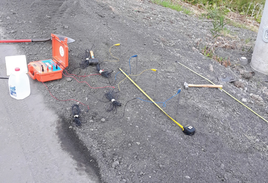
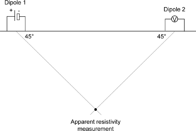
Electrical resistivity methods are commonly applied in the field. The field measurement of resistivity is similar to the laboratory method described above but at a different scale. In a simple arrangement, four electrodes are coupled to the ground via stainless steel stakes and aligned linearly to obtain data (see Figure 6.1). Two of the electrodes induce electric current in the subsurface (which generates an electric field), and two electrodes measure the resulting voltage potential. Electrical resistivity in the field typically is reported in ohm-meters, as opposed to ohm-centimeters reported in laboratory units, due to the relatively larger magnitude of resistivity of some subsurface materials, such as porous rocks (e.g., limestone). The average depth of each apparent resistivity data point is a function of the arrangement of the electrodes at the surface, most notably the distance between the current and
___________________
1 Soils in earth retention systems are considered nonaggressive if they have resistivities of more than 3,000 ohm-cm; and soils around nonmarine piles are considered nonaggressive if they have resistivities of more than 2,000 ohm-cm (AASHTO, 2002).
SOURCE: K. Fishman, committee member.
voltage pairs (see Figure 6.2). The term “apparent” is used to denote that each measurement assumes that the earth is homogeneous. When only four electrodes are used that are relatively close together (i.e., less than 0.5 m apart as in Figure 6.1) and only one apparent electrical resistivity measurement is collected, this assumption is reasonable for the relative volume of soil tested, and the apparent resistivity is assumed to be the true electrical resistivity. Although soil is a heterogeneous material, electrical resistivity is a bulk measurement that cannot discern small changes in the three phases of soils. However, other surveys using many electrodes test a much larger volume of soil, in which case each apparent electrical resistivity measurement likely includes much more significant changes in the three phases (i.e., several different soil layers or the groundwater table). For these measurements, the apparent resistivity cannot be assumed to equal the true resistivity and thus they require more extensive modeling. These multielectrode surveys can also be used for three-dimensional models.
Various complementary laboratory and field resistivity methods have been established (e.g., ASTM G57-20, 2020; ASTM G187-18, 2018) and theoretically should yield the same resistivity. However, given that the moisture content of the sample as received in the laboratory will be different than in situ, it is often difficult to correlate laboratory and field resistivity measurements (see Box 6.4). Some field data acquisition equipment allows a linear array of more than four electrodes and multiple voltage measurements at once, reducing data collection time when the objective is to cover a larger area. The data then are converted to a two-dimensional plot of apparent resistivity, and the true resistivity distribution of the subsurface is obtained through an inversion process. Note that there are inherent limitations to directly using multielectrode field resistivity measurements to determine soil corrosivity,
particularly with depth, as the granularity of the inversion process required to interpret field electrical resistivity measurements does not represent the same discrete volume of soil measured in the laboratory. Although application of both finite element and applied element methods to data inversion can reduce artifacts and excessive smoothing, neither technique is perfect. So, while field methods for determining subsurface electrical resistivity exist and are increasingly popular in geo-civil industries, they are not a common standard practice for evaluating corrosivity.
Electromagnetic Induction
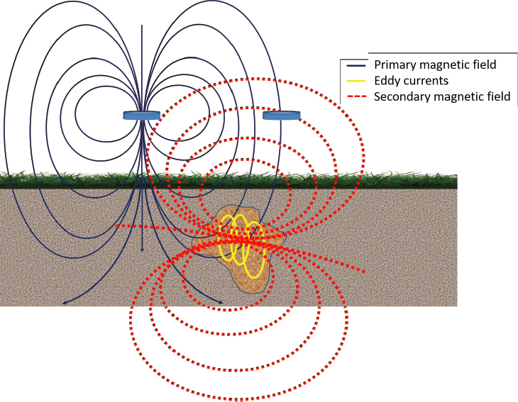
Electrical conductivity (or its inverse, electrical resistivity) can also be measured via EMI, a noncontact (i.e., inductive) geophysical method in which the mutual impedance between two or more coils at or above the ground surface, or downhole, is measured. The general method begins with a time-dependent electric current flowing in
a transmitter coil, which generates a transient primary magnetic field. This field expands outward, and part of it will flow into the subsurface, which generates an electromotive force and causes eddy currents to flow (see Figure 6.3). The eddy currents generate a secondary magnetic field, which is influenced by the characteristics of the subsurface, namely, the subsurface conductivity. The receiver coil senses both the primary and secondary magnetic fields. The bulk apparent electrical conductivity is determined from the measured primary and secondary fields and is typically reported in millisiemens per meter (mS/m; 1 mS/m = 1,000 ohm-m). Inversion modeling of EMI data is necessary to obtain true electrical conductivity values, but this is rarely done. EMI data are typically used to quickly identify changes in bulk conductivity to indicate, for example, where further investigation is warranted or excavation might prove useful. The apparent depth of the measurement is estimated from the conductivity of the soil, the EMI sensor frequency, and the sensor height above the ground. The term “apparent” indicates that the depth is not a true measurement but rather an estimated measurement based on the assumption that the subsurface is homogeneous.
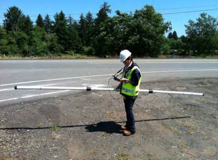
EMI measurements are commonly used by the oil and gas pipeline industry or for other applications where continuous data along long linear structures are desirable. The commercially available, noncontact devices used for EMI allow for fast and easy data collection over relatively large distances. For example, a person carrying the device can walk with (see Figure 6.4) or drag a sensor via a sled behind a vehicle and set the device to collect data linked with global positioning system locations every few seconds along a pipeline corridor and rapidly collect continuous apparent electrical conductivity measurements.
Assessing Impact of Stray Currents
As discussed in Chapter 2, stray electrical currents may exist around direct current (DC) mass transit facilities, electrical transmission systems, waterfront structures in saltwater, cathodic protection systems, or welding shops,
SOURCE: Saquib Mohammed Haroon, modified with permission.
SOURCE: Mersedeh Akhoondan, committee member.
and may affect buried utility pipes and cables, underground storage containers, and reinforced concrete structures, particularly in high-density urban areas. In general, stray currents rapidly decrease in magnitude away from their source and are not a risk 100 to 200 feet away from the source. Examples of characterizing subsurface stray currents include identifying the distribution of potential gradients between the current source and buried steel of interest. The source might be stray-current leakage from, for example, DC-powered transit systems (Sankey and Hutchinson, 2011). The gradient is a function of rail track-to-earth potential (i.e., between the track and earth) and resistance and can be estimated by measuring earth electrical gradients near the source of the stray current. In contrast, the interference of aerial high-voltage alternating current (AC) power lines on colocated (i.e., nearby) pipelines can be assessed using properties such as the proximity and spatial arrangement of steel and high-voltage AC traveling through the power line and soil resistivity. Finneran et al. (2015) developed a screening tool to identify the conditions under which more resource-intensive analyses and modeling related to stray currents are warranted. Table 6.6 provides simplified examples of the factors, thresholds, and severity rankings they identified; the table also provides some values to consider. Finneran et al. (2015) provide far more detail regarding these and other factors. Their screening tool identifies the severity of risk of high-voltage AC interference with colocated pipeline based on different combinations of factors such as those listed in Table 6.6.
As with any characterization methodology, there is a certain amount of uncertainty associated with the characterization of stray currents and their possible impacts. The difficulty characterizing the subsurface for corrosivity has been described above, and each method, such as determination of resistivity, has its own uncertainties. Cumulative error may be generated using a screening tool such as described by Finneran et al. (2015) because of the uncertainties associated with each factor contributing to the risk assessment. When using such tools, it is important to understand how the tools were developed (e.g., are they empirically or model based?) so that reasonable judgment may be applied with respect to the significance of the results obtained from them. Further complicating characterization of how stray currents affect buried steel infrastructure, if all stray currents and their sources are even known, is the fact that the owners or operators of stray-current sources (e.g., power companies or rail services) will likely be different than the owners or operators of the steel infrastructure. It could be difficult obtaining, for example, the exact location or amperage of the stray-current source.
TABLE 6.6 Examples of Threshold Rankings of Severity of Interference of High-Voltage Alternating Current Power Lines and Pipelines
| Example Factors and Thresholds | Ranking of Severity of Interference |
|---|---|
| Separation distance from high-voltage alternating current source | |
| Less than 100 feet | High severity |
| Greater than 1,000 feet | Very low severity |
| Power line current | |
| Greater than 1,000 amps | Very high severity |
| Between 500 and 1,000 amps | High severity |
| Less than 100 amps | Low severity |
| Soil resistivity | |
| Less than 2,500 ohm-cm (laboratory measurement) | Very high severity |
| Greater than 30,000 ohm-cm (laboratory measurement) | Low severity |
| Colocation length | |
| Greater than 5,000 feet | High severity |
| Less than 1,000 feet | Low severity |
| Colocation crossing angle | |
| Less than 30 degrees | High severity |
| Greater than 60 degrees | Low severity |
NOTES: These are examples considered by Finneran et al. (2015). Note that they considered how the combination of factors at specific threshold should trigger more rigorous analysis.
Assessing the Risk of Microbially Influenced Corrosion
Some projects, including large bridge projects, have attempted to use microbial culture (growth) testing to estimate the viable populations of specific bacteria in a given environment. However, these tests are generally unsuitable for assessing the risk of future microbial attacks given the ubiquity of some microbes and the inability to cultivate all species. Instead, projects are more commonly assessed for the likelihood of microbially influenced corrosion (MIC) using subsurface properties. However, those properties that make an environment particularly susceptible to MIC are still debated, and some soil properties are even a consequence of microbial activities. Agarry and Salam (2016) reported that low redox potential and poor drainage due to fine grain size (e.g., clay and silt) were favorable to sulfate-reducing bacteria (SRB), whereas Li et al. (2001) determined that acid-producing bacteria (APB), total organic carbon, resistivity, and water content (listed in descending order of importance) were important. In contrast, Jansen et al. (2017) concluded that the most important properties were sulfate reduction (redox potential, organic matter, and sulfate), mass transfer, and changing conditions (introduction of oxygen or nitrate).
Several standard practices require additional corrosion protection when the subsurface is deemed to be particularly susceptible to future MIC. The Association for Materials Protection and Performance (AMPP) and the American Petroleum Institute (API) require the implementation of specialized measures to prevent MIC when the soil has sulfate concentrations in excess of 500 parts per million (NACE Committee TEG 187X, 2019). AMPP and API also provide some guidance regarding cathodic protection for underground steel piping when MIC is likely (NACE SP0169, 20132). In contrast, ASTM International recommends that redox potential measurements be used to determine the propensity for MIC (ASTM G 200-20, 2020). It states that soils with negative redox potentials are considered severely corrosive, whereas soils with redox potentials exceeding 100 mV are considered noncorrosive. Despite these standard practices, assessing the likelihood of MIC remains difficult because stratified biofilms can often create highly localized conditions that may not reflect highly averaged field surveys of heterogeneous sub-surfaces or even samples of soils taken for laboratory analysis. Additionally, the type of infrastructure may affect the susceptibility to MIC (see Box 6.5). Cathodic protection, common on oil and gas pipelines and some water
___________________
2 Section 6.2.1.4.1 states, “When active MIC has been identified or is probable (e.g., caused by acid-producing or sulfate-reducing bacteria), the criteria listed in Paragraphs 6.2.1.2 and 6.2.1.3 might not be sufficient.”
pipelines, alters the soil environment at the soil–pipe interface that may influence the types, numbers, and activities of soil microorganisms. In addition, many of the legacy coatings used on oil and gas pipelines are biodegradable. Leaks in water distribution systems, which may be ignored from a safety perspective, can contribute oxygenated, treated water to otherwise dry, anaerobic pipe–soil interfaces.
STANDARD PRACTICE DURING OPERATIONS AND AFTER FAILURE
Subsurface characterization after the initial site investigation is not routinely performed as part of operation and maintenance of facilities with buried steel within the geo-civil industries. Observations of external conditions may be documented over time by maintenance personnel or during broader inspection programs during which wet areas, vegetation growing from unintended places (e.g., the face of a retaining wall), rust stains appearing on the facing of a wall system, or poor drainage conditions might be observed. Such observations could inform decisions related to maintenance operations (e.g., to improve drainage) and the need for further evaluation (e.g., exposing buried steel to directly observe conditions) or rehabilitation. Additional subsurface characterization may be undertaken after unexpected metal loss has been observed on exposed steel. This may occur during a retrofit or as construction proceeds to modify an existing facility but is not performed as routine maintenance and operations. Older buried steel may be exposed as an existing facility is demolished or excavated as part of an improvement project. Investigations to determine the cause of observed accelerated corrosion are often conducted, and these include identifying subsurface conditions and measurements of soil properties and characteristics including salt content, resistivity, pH, organics, and moisture content. Samples are obtained from different depths and locations within the subsurface along the facility. Bulk samples from near the surface (to depths of approximately 5 feet) may be obtained from test pits, and samples from deeper depths may be obtained via an auger equipped with a split spoon sampler or in some cases by coring though the face of an existing retaining wall.
More substantial subsurface characterization will occur after a failure. Failure can take various forms but includes observations of unexpected movement of an MSE wall, vertical movement of a bridge pier, soil movement as evidenced by a soil surface depression, or in some cases, catastrophic failure of a structure or portion of a structure. In these cases, there will likely be a forensic investigation into the probable cause of an observed issue, which may include characterization of the current conditions of the underlying soil of a supported structure or soil fill behind a wall. The failure of embedded steel elements due to corrosion should be explored as a possible reason for a failure. When available, geotechnical information from original construction can be useful in examining possible changes in the subsurface environment that may have led to corrosion. As part of a forensic subsurface characterization, soil samples with depth will be taken. This is typically accomplished using standard geotechnical sampling techniques. Unexpected types of soil or fill materials of significant depth or layer could be a sign of inappropriate dumping of materials during original construction. During sampling, the height of the
water table should be noted to understand possible environmental factors that can be associated with corrosion. Soil samples can be tested to characterize corrosivity by measuring resistivity. Chemical analysis of contaminants in the soil such as chlorides, sulfates, or other corrosive species should be performed to measure concentrations of these corrosive species.
Because of the damage that can occur from failures, many oil and gas pipelines are required by regulation to periodically monitor and inspect for the integrity of the asset. While many technologies exist to help identify the areas most likely to need repair or remediation (see Chapter 7), the relatively shallow placement (usually about 3 feet deep) of pipelines allows for direct inspection or forensic investigation. As such, these pipeline “digs” will often include obtaining a soil sample at the point of contact with the pipeline and any associated corrosion identified to characterize any constituents that may have exacerbated the condition. Resistivities, chlorides, sulfates, and microorganisms are examples of the types of properties that are evaluated to determine whether cathodic protection and a reapplication of protective coating is needed.
Standard Practice for Characterizing Microbially Influenced Corrosion During Operations and After Failure
Detailed test methods for diagnosing MIC after it has occurred are available (NACE TM0106, 2016), but early detection of MIC is difficult. MIC can be monitored using coupons that can be easily removed and visually inspected. The presence of slime, odors, and pitting may be indicative of MIC (Little et al., 2020). Coupons can be removed and further examined using other diagnostic methods. MIC diagnostic methods rely on quantifying specific groups of microorganisms, especially bacteria, or some constitutive property (e.g., deoxyribonucleic acid [DNA], ribonucleic acid [RNA], and adenosine triphosphate [ATP]). DNA can be isolated from active and inactive cells and can remain intact after cells are dead. Both RNA and ATP are constituents of active cells.
The traditional method for detecting groups of bacteria associated with MIC is the serial dilution-to-extinction method. This uses culture media designed to grow specific microorganisms (e.g., SRB or APB) (Little and Lee, 2007). Tenfold dilutions of either solutions or buffered suspensions of solids (e.g., soil or corrosion products) in diagnostic media are used to estimate population sizes. Growth is detected as turbidity or a color change, which indicates a chemical reaction. The method is based on the premise that a single cell will produce a reaction in the culture medium. Consequently, small numbers of cells can be detected. However, large numbers of cells require multiple dilutions. The goal is to dilute to the point that bacteria are no longer detectable in a sample (i.e., extinction). Estimated population size is reported as the highest dilution to produce a positive result (e.g., a dilution of 103). Commercial test kits for use in the laboratory or field are available with explicit directions for sample collection, inoculation, and interpretation. All culture media are selective to specific organisms and do not account for the nonculturable organisms. Kieft (2000) estimated that only 0.001 to 4 percent of soil microorganisms could be cultured on organic growth media. Therefore, results from culture techniques can provide misleading results—both false positives and false negatives. Furthermore, most commercially available test kits are designed to enumerate bacteria and do not account for fungi or archaea. These respective groups can influence corrosion of carbon steel by organic acid and sulfide production, respectively.
To address issues related to culture techniques, more recent MIC diagnostic efforts have focused on molecular microbiological methods. Hybridization techniques (e.g., fluorescence in situ hybridization [FISH] and DNA arrays) use probes (i.e., DNA fragments designed to bind to DNA or RNA from specific microorganisms [Shakoori, 2017]). FISH probes can be designed to target total bacteria, archaea, or specific groups (e.g., SRB). Only active cells are stained with the fluorescent dye. In contrast, polymerase chain reaction (PCR) can be used to synthesize and amplify a specific section of DNA with a “primer” or “probe” (e.g., targeting the 16S ribosomal RNA gene; Klindworth et al., 2013). Following PCR, the amplified regions are sequenced and used to identify microorganisms. However, unlike hybridization techniques, PCR does not distinguish between DNA from live and dead cells. This is problematic because extracellular DNA (e-DNA), which is DNA that occurs outside of living organisms, may be the largest fraction of total DNA in some environments. Extracellular DNA and DNA from dead cells indicate that there is no direct link between a characterized DNA pool and actual living microbial cell abundance and diversity in a sample (Eid et al., 2018; Makama et al., 2018). Reverse transcription of RNA followed by PCR or quantitative PCR is a PCR-based approach to quantify active cells. However, the design of
probes and primers in the PCR techniques requires prior knowledge about the microorganisms in the sample. Most important, numbers of bacterial cells as determined by any method and MIC kinetics have not been correlated. In some circumstances, low numbers of microorganisms could be responsible for severe corrosion, and in other circumstances, large numbers of the same organisms may not be related to corrosion (Little et al., 2020). Therefore, microbial quantification only indicates the extent of microbial presence but does not allow for estimation of the role of microorganisms in corrosion processes.
EMERGING PRACTICES: USE OF DECISION SUPPORT TOOLS
Many laboratory standards evaluate the properties of soils using a specific size fraction. For example, a standard test for resistivity developed by AASHTO (AASHTO T 288-12, 2016) is performed on the fine-grained sample fraction that passes a 2-mm sieve (i.e., No. 10 sieve). The test focuses on fine-grained material because electrical current will travel along paths where lower-resistance fine material is concentrated, meaning that corrosivity is controlled more by the properties of the finer portions than by the bulk portions of the material. Therefore, the test only accurately reflects the subsurface when the sample collected has a significant fraction of fine-grained material. Measurements of corrosion rates (estimated from weight loss and thickness measurements) and resistivity from North American and European sites are available from a database catalogued as part of National Cooperative Highway Research Program 24-28 (Fishman and Withiam, 2011). Fishman et al. (2021) culled the Fishman and Withiam (2011) data such that coarse samples with less than 22 wt % smaller than 2 mm were removed from the dataset. The culled data are presented in Figure 6.5a compared with data that are not discriminated based on the coarseness of the sample in Figure 6.5b. The report concluded that AASHTO T 288-12 (2016) is only appropriate for measuring resistivity for materials where greater than 22 wt % of particles are less than 2 mm. For material where less than 22 wt % of particles are smaller than 2 mm, other standards that test the material in its “as-received gradation” were considered more appropriate (e.g., Arciniega et al., 2021).
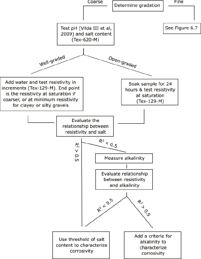
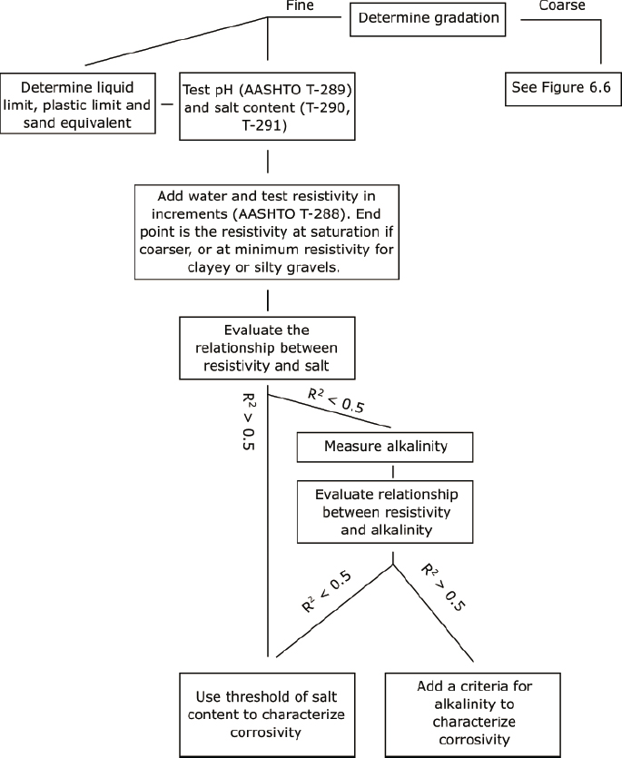
Fishman et al. (2021) attempted to improve methods for characterizing the corrosivity of earth materials by creating a proposed protocol for sampling, testing, and characterizing earth materials (described in flowcharts in Figures 6.6 and 6.7). This simple decision flowchart can be used to determine if the procedures described by Arciniega et al. (2021)—samples tested in “as-received gradation”—or the AASHTO procedures (samples tested after separation on a 2-mm [i.e., No. 10] sieve) will be more accurate given the gradation of the sample. The flowchart begins with determining the particle sizes of the material (i.e., soil gradation). Flowcharts and decision-making tools have been used for many years, including in NCHRP Report 408 (Beavers and Durr, 1998) and AASHTO R 27 (2001), which describe decision support system (DSS) tools for making decisions about data collection, design, and monitoring for corrosion of steel piles, as well as NCHRP Report 477 (Withiam et al., 2002). The latter provides a recommended practice for service-life modeling of ground anchorages. More detailed variations of such DSSs could be developed and made available in the future to guide decisions in a variety of corrosion-related practices. One example of a Web-based DSS is offered through the Geo-Institute of the American Society of Civil Engineers.3 GeotechTools is a decision-making tool that identifies suggested technologies for specific construction applications using project information and constraints, such as the type of application and the purpose of the technology. For example, a selected application of “construction on unstable soils” for the purpose of “compaction” on GeotechTools.org results in a number of suggested techniques (traditional compaction, intelligent compaction, rapid-impact compactor, or high-impact rollers) and presents information about the establishment or maturity of that technology.
ASPIRATIONAL BIOCEMENTATION METHODS FOR CONTROL OF ENVIRONMENT
Biocementation is an aspirational technology that could impact corrosion of buried steel structures. Bacteria-mediated calcium carbonate (CaCO3) precipitation is a ground improvement technique that requires an external
___________________
3 See https://www.geoinstitute.org/geotechtools/login (accessed June 21, 2022).
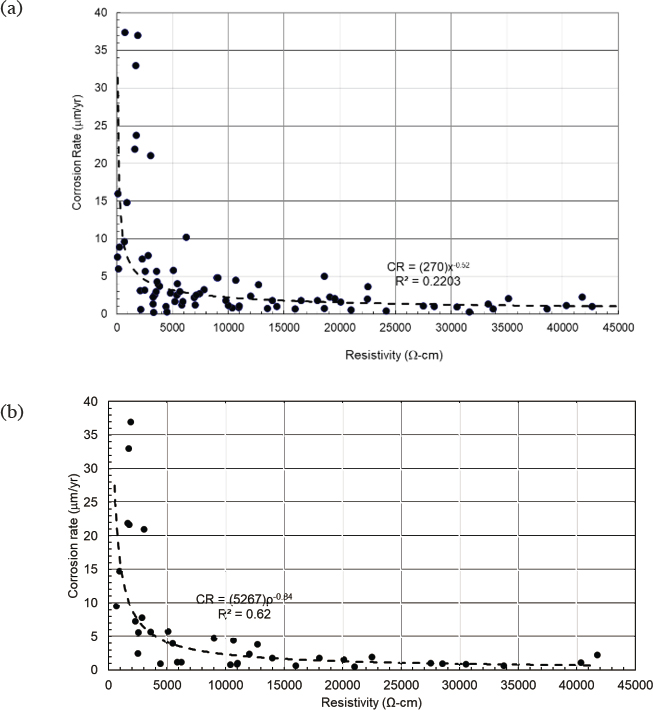
SOURCES: Fishman and Withiam (2011); Fishman et al. (2021).
source of calcium and is designed to decrease the permeability and increase stability of soils (Mujah et al., 2017; Umar et al., 2016). Some bacteria, particularly those that break down urea (ureolytic bacteria), influence the precipitation of CaCO3 by the production of the urease enzyme. Hydrolysis of urea by urease produces carbon dioxide (CO2) and ammonia (NH4), increasing the pH and precipitating CaCO3. Biocementation has been used in a variety of geotechnical engineering applications (Ferris et al., 1996; Whiffin et al., 2007) in both sandy (Nemati and Voordouw, 2003) and organic soils (Sidik et al., 2014). Biocementation coats or bridges individual soil particles, gradually reducing the pore size within the soil fabric, and reducing the hydraulic conductivity. Despite the relative efficiency of ureolysis compared to other possible pathways for biocementation, there are some challenges, including environmental challenges associated with the high production of ammonia during the breakdown of urea (Al-Thawadi, 2011). However, as research continues, methods such as this might prove viable for precipitating a corrosion-resistant coating on buried steel at scales relevant to buried steel infrastructure.
SOURCE: Adapted from Fishman et al. (2021).
SOURCE: Adapted from Fishman et al. (2021).


