
Solid-Fluid Juncture Boundary Layer and Wake with Waves
J.E.Choi and F.Stern
(University of Iowa, USA)
ABSTRACT
Laminar and turbulent solutions are presented for the Stokes-wave/flat-plate boundary -layer and wake for small-large wave steepness, including exact and approximate treatments of the free-surface boundary conditions. The macro-scale flow exhibits the wave-induced pressure-gradient effects described in precursory work. For laminar flow, the micro-scale flow indicates that the free-surface boundary conditions have a profound influence over the boundary layer and near and intermediate wake: the wave elevation and slopes correlate with the depthwise velocity; the streamwise and transverse velocities and vorticity display large variations, including islands of maximum/minimum values, whereas the depthwise velocity and pressure indicate small variations; significant free-surface vorticity flux and complex vorticity transport are displayed; wave-induced effects normalized by wave steepness are larger for small steepness with the exception of wave-induced separation; order-of-magnitude estimates are confirmed; and appreciable errors are introduced through approximations to the free-surface boundary conditions. For turbulent flow, the results are similar, but preliminary due to the present uncertainty in appropriate treatment of the turbulence free-surface boundary conditions and meniscus boundary layer.
NOMENCLATURE
|
A |
=wave amplitude |
|
Ak |
=wave steepness |
|
Fr |
=Froude number |
|
g |
=gravitational acceleration |
|
k |
=turbulent kinetic energy |
|
=wave number |
|
|
L |
=body characteristic length |
|
n |
=unit normal vector |
|
o( ), ( ) |
=order of magnitude |
|
p |
=piezometric pressure |
|
p* |
=static pressure |
|
q |
=free-surface vorticity flux (=qx,qy,qz) |
|
qw |
=wall vorticity flux (=qwx,qwy,qwz) |
|
Re |
=Reynolds number (=UoL/v) |
|
u,v,w |
=fluctuating velocities |
|
|
=reference velocity |
|
−uiuj |
=Reynolds shear stresses |
|
V |
=mean-velocity vector (= U,V,W) |
|
x,y,z |
=Cartesian coordinates |
|
δ |
=body (δb) or free-surface (δfs) boundary-layer or wake (δW) thickness |
|
δ* |
=streamwise displacement thickness |
|
Δ |
=difference between zero and nonzero wave-steepness values of |
|
ε |
=rate of turbulent energy dissipation |
|
=boundary-layer and wake thickness |
|
|
|
=transport quantities (= U,V,W,k,ε) |
|
=relevant variable or equation |
|
|
η |
=wave elevation |
|
λ |
=wave length |
|
μ |
=viscosity |
|
v |
=kinematic viscosity (=μ/ρ) |
|
ρ |
=density |
|
|
=wall-shear stress |
|
|
=fluid stress tensor |
|
|
=external stress tensor |
|
ξ,η,ζ |
=nonorthogonal curvilinear coordinates |
|
ω |
=mean vorticity vector (=ωx,ωy,ωz) |
INTRODUCTION
Ship boundary layers and wakes (blw's) are unique in that they are influenced by the presence of the free-surface and gravity waves. The wave pattern, breaking, and -induced separations along with turbulence/vortex/free-surface interaction, bubble entrainment, etc. are key issues with regard to performance prediction, signature reduction, and propeller-hull interaction.
In spite of this, until fairly recently, very little detailed experimental or rigorous theoretical work has been done on this problem. In
particular, over the past ten years, the Iowa Institute of Hydraulic Research (IIHR) has carried out an extensive experimental and theoretical program of research concerning free-surface effects on ship blw' s: problem formulation and model problem identification [Stokes-wave/flat-plate (Sw/fp) flow field] and calculations [1]; towing-tank experiments for idealized (foil-plate model which simulates the Sw/fp flow field) and practical hull form (Series 60 CB=.6) geometries [2–5]; and the development of computational fluid dynamics (cfd) methods, including validation studies for the foil-plate model [3] and Wigley [6] and Series 60 CB=.6 [7] hull forms. Through this work, significant progress has been made in explicating certain features of the flow physics (e.g., wave/blw interaction, including the role of wave-induced pressure gradients, wave-induced separation, and scale-effects on near-field wave patterns) and identifying issues for further study (e.g., the nature of the flow very close to the free surface, including the role of the free-surface boundary conditions and the structure of turbulence, effects of geometry and turbulence on wave-induced separation, wake bias, and pacesetting issues for cfd advancements).
This paper concerns one of the aforementioned issues for further study, i.e., the nature of the flow very close to the free surface, including the role of the free-surface boundary conditions. Laminar-flow solutions are presented for the Sw/fp flow field, including the exact free-surface boundary conditions. The work presents for the first time solutions to the exact governing Navier-Stokes (NS) equations and boundary conditions for a solid-fluid juncture blw with waves. Some additional turbulent-flow solutions are also presented; however, these are preliminary due to the current uncertainty in prescribing appropriate turbulence free-surface boundary conditions and treatment of the meniscus boundary layer.
The complete results are extensive and provided by Choi [8]. In the following, the most important aspects of the solutions are discussed and example results are presented. First, overviews are given of the physical problem, including order-of-magnitude estimates (ome), and precursory and relevant work, and the computational method. Then the computational conditions, grids, and uncertainty are described and results presented and/or discussed for small, medium, and large wave-steepness Ak (where A and k are the wave amplitude and number, respectively) for laminar and turbulent flow. Lastly, a summary and conclusions are made, including recommendations for future study and implications with regard to practical applications.
PHYSICAL PROBLEM AND PRECURSORY WORK
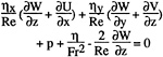
Consider the development of the blw for a ship moving steadily at velocity Uo in an incompressible viscous fluid (figure 1). Following [1], the flow in the neighborhood of the body blw/free-surface juncture is divided into five regions (figure 2): (I) potential flow; (II) free-surface boundary layer; (III) body blw; (IV) solid-fluid juncture blw with waves; and (V) meniscus boundary layer.
The flow in region I is well known, i.e., ome and analytical and cfd methods are well established. The situation is similar for region II, at least for laminar flow, e.g., the analytical solution provided in Appendix A of [8]. Table 1 of [8] provides inviscid and viscous Stokes-wave solutions for regions I and II. In region III, the effects of the free surface are primarily transmitted through the external-flow pressure field and, here again, ome and cfd methods are available. The precursory work mentioned earlier and described later has been very successful in documenting the nature of the flow in this region. In region IV, the effects of the free surface are due both to the influences of the external-flow pressure field and the kinematic and dynamic requirements of the free-surface boundary conditions, which alters both the mean and turbulent velocity components. Presently, the only available information for region IV is that provided by [1], i.e., ome and preliminary calculations for the Sw/fp flow field, including approximate free-surface boundary conditions. Some relevant work, which is also useful in understanding the flow in region IV is described later. Region IV is the topic of this paper. The flow in region V is presently poorly understood, involving surface-tension and contact-line effects. Region V is neglected in this paper, but, as discussed later, recommended for future study.
Order-of-Magnitude Estimates
[1] provides a discussion of the ome for regions I through III and a derivation for those for region IV in connection with the determination of appropriate small-amplitude-wave and more approximate free-surface boundary conditions. In regions I through III, the important nondimensional parameters are Ak and Reynolds number (Re) or related blw thickness ε=δ/L or δ/λ (where δ is the body or free-surface boundary-layer or wake thickness, δb, δfs, δW, respectively, L is the body characteristic length, and λ=2π/k is the wave length). For sufficiently
large Re and slender bodies, the ome for regions I through III in terms of these parameters are provided in table 1. In region IV, the ome were derived in consideration of both those for region III, with the assumption of thin-boundary-layer theory, and the requirements of the free-surface boundary conditions. Additionally, Ak/Ɛ is shown to be an important parameter. However, the assumption of thin-boundary-layer theory for region III led to an error for one of the estimates, i.e., Wz1; therefore, an updated derivation is provided as follows.
In consideration of the flow in regions I and III, the ome for V=(U,V,W), η, ∂/∂x, and ∂/∂y are:
V=(1,ε,Ak)
η=(Ak)
∂/∂x=(1)
∂/∂y=(ε−1) (1)
Next, the normal and tangential dynamic and continuity-equation free-surface boundary conditions (see later), respectively
(2)

(3)

(4)
(5)
are used, i.e., using (3)–(5), respectively, to eliminate Uz, Vz, and Wz in (2), solving for p, and with (1) results in the ome for p:
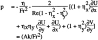
(6)
Finally, using (3)–(5) with (1) and (6) results in the ome for Uz, Vz, and Wz, respectively:

(7)

(8)
(9)
The ome for region IV are provided in table 1 and, as will be shown later, are confirmed by the present results. Note that the only differences with those provided previously by [1] are for Wz, as mentioned earlier, and that a single estimate is not provided for ∂/∂z.
Thus far, no distinction has been made between the flow in the blw regions, which is not necessary, except for the far-wake (fw) region, i.e., hereafter, the blw refers to the boundary-layer and near- and intermediate-wake in distinction from the fw. The fw requires a different ome derivation. In this case, in consideration of the flow in region I and the asymptotic two-dimensional zero-pressure gradient fw solution [9], the ome for V, ∂U, η, ηx, ηy, ∂/∂x, and ∂/∂y are:

(10)
Next, following the usual derivation for region III both for the blw and a similar derivation as provided earlier for region IV both for the blw, the ome for regions III and IV for the fw are derived. These are also provided in table 1 and, here again, as will be shown later, are confirmed by the present results.
|
1 |
Subscripts are used to denote derivatives, as indicated here, or in defining certain variables, as indicated in the Nomenclature. |
Regions III Calculations and Experiments
[1] identified the model problem of a combination Sw/fp flow field (figure 3), which facilitated the isolation and identification of the most important features of the wave-induced effects. Numerical results were presented for laminar and turbulent flow utilizing first-order boundary-layer equations and both small-amplitude-wave and more approximate zero-gradient free-surface boundary conditions. Subsequently [2], results from a towing-tank experiment were presented utilizing a unique, simple foil-plate model geometry, which simulates the Sw/fp flow field. Mean-velocity profiles in the boundary-layer region and wave profiles on the plate were measured for three wave-steepness conditions. For medium and large steepness, the variations of the external-flow pressure gradients were shown to cause acceleration and deceleration phases of the streamwise velocity component and alternating direction of the crossflow, which resulted in large oscillations of the displacement thickness and wall-shear stress as compared to the zero-steepness condition. The measurements were compared and close agreement was demonstrated with the results from the turbulent-flow calculations with the zero-gradient approximation for the free-surface boundary conditions. Also, wave-induced separation was discussed, which was present in the experiments, and the starting point was predicted by the laminar-flow calculations under certain conditions.
More recently [3], results were presented from extensions of both the previous experimental and theoretical work: the measurement region was extended into the wake where both mean-velocity and wave-elevation measurements were made; and a state-of-the-art cfd method was brought to bear on the present problem, in which the Reynolds-averaged NS (RaNS) equations were solved for the blw region with zero-gradient free-surface boundary conditions. Measurements and calculations were performed for the same three wave-steepness conditions. The trends were even more pronounced for the wake than shown previously for the boundary-layer region. Remarkably, the near and intermediate wake displayed a greater response, i.e., a bias with regard to favorable as compared to adverse pressure gradients [8]. The measurements were compared and close agreement was demonstrated with results from the RaNS calculations. Additional calculations were presented, including laminar-flow results, which aided in explicating the characteristics of the near and intermediate wake, the periodic nature of the fw, and wave-induced separation.
Very little is known about wave-induced separation, i.e., three-dimensional boundary-layer separation near the free-surface induced by waves and accompanied by a large disturbance to the free surface itself. The additional laminar-flow computational results of [3] enabled, for the first time, a detailed study, including the flow pattern in the separation region. A saddle point of separation and a focal point of attachment were indicated on the plate and mean free surface, respectively. As the wave steepness increased, the saddle point moved downwards and towards the trailing edge, whereas the focal point moved downstream and away from the plate surface. The U and W components displayed, respectively, flow reversal and complex S-shaped profiles. A longitudinal vortex was generated in which the vortical motion was counterclockwise with respect to the flow direction and towards the free surface and clockwise with respect to the flow direction and in the main stream direction above (i.e., in the reverse-flow region) and below the saddle point, respectively. The identification of these features of wave-induced separation was considered very significant and invaluable, but with some caution and to some extent preliminary due to the approximate nature of the free-surface boundary conditions used in the calculations. This paper also addresses this issue.
RELEVANT WORK
Relevant work concerns viscous-free-surface flow, i.e., solutions of the viscous-flow equations, including various treatments of the free-surface boundary conditions, for a variety of applications, i.e: free-wave problems, open-channel flow, free-surface jet flow, vortex/free-surface interaction, and ship blw's for nonzero Froude number (Fr). In [8], the critical issues with regard to the implementation of the free-surface boundary conditions and the various treatments utilized are discussed. Also, for the latter applications, the most important results are summarized both with regard to experimental information and physical understanding and computational studies. The discussions are useful for the evaluation and interpretation of the present solutions with regard to their significance and the role of the free-surface boundary conditions. The conclusions with regard to the relevant work are summarized as follows (see [8] for references).
A variety of cfd formulations of viscous-free-surface flow are possible with the ability to predict a wide class of flows; however, none have fully implemented the free-surface boundary
conditions or resolved the free-surface boundary layer and taken into account complicating factors such as the meniscus boundary layer, etc. Turbulence free-surface interaction has been investigated for certain idealized geometries (i.e., open-channel flow, free-surface jet flow, and a submerged tip vortex) all of which indicate similar free-surface effects: constant turbulent kinetic energy (i.e., zero gradient) with a redistribution of energy between the turbulence velocity components, i.e., the vertical turbulence velocity is damped and the horizontal and streamwise components are increased. Free-surface jet flow also displays effects due to jet-induced waves and free-surface induced lateral spreading. The idealized geometries are different than ship blw's in that the source of turbulence does not pierce the free surface and the role of gravity waves is minimal. Considerable experimental and computational information is available for vortex/free-surface interaction for laminar flow and clean free surfaces, which indicates complex features involving interrelated free-surface deformation, secondary-vorticity generation, and vorticity reconnection; however, a complete understanding of the physics is lacking, i.e., most studies are descriptive and controversey exists as to the physical mechanisms. The role of surfactants and turbulence are insufficiently understood. Although certain progress has been made in the understanding of the practical application of ship blw's for nonzero Fr, the detailed flow structures, including turbulence and the micro-scale flow are poorly understood.
COMPUTATIONAL METHOD
The computational method is based on extensions of [3] for region IV calculations, including the use of a two-layer k-ε turbulence model [10]. [3] is a modified version of the large-domain viscous-flow method of [11] for small-domain calculations and free-surface boundary conditions. Only a brief review of the basic viscous-flow method is provided, but with a detailed description of the present solution domain and boundary conditions. Further details are provided in [8] as well as [10,11] and associated references.
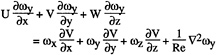
In the viscous-flow method, the RaNS equations are written in the physical domain using Cartesian coordinates (x,y,z). For laminar-flow calculations, the equations reduce to the NS equations by simply deleting the Reynolds-stress terms and interpreting (U,V,W) and p as instantaneous values. The governing equations are transformed into nonorthogonal curvilinear coordinates (ξ,η,ζ) such that the computational domain forms a simple rectangular parallelepiped with equal grid spacing. The transformation is a partial one since it involves the coordinates only and not the velocity components (U,V,W). The transformed equations are reduced to algebraic form through the use of the finite-analytic method. The velocity-pressure coupling is accomplished using a two-step iterative procedure involving the continuity equation based on the SIMPLER algorithm. Both fixed and free-surface conforming grids were used for the calculations. In both cases, a simple algebraic technique was used whereby the longitudinal and transverse sections of the computational domain are surfaces of constant ξ and η, respectively; and, moreover, the three-dimensional grids were obtained by simply “stacking ” the two-dimensional grid for the transverse plane.
The Sw/fp solution domain and coordinate system are shown in figure 3. In terms of the notation of figure 3, the boundary conditions are as follows. On the inlet plane Si, ![]() is specified from the Stokes-wave solutions (i.e., table 1 of [8]) and typical free-stream values for (k,ε). On the body surface Sb, the no-slip condition is imposed. On the symmetry planes Scpand Sd, ∂(U,W,p,k,ε)∂y=V=0 and ∂(U,V,p,k,ε)/∂z=W =0, respectively. On the exit plane Se, axial diffusion is negligible so that ∂2
is specified from the Stokes-wave solutions (i.e., table 1 of [8]) and typical free-stream values for (k,ε). On the body surface Sb, the no-slip condition is imposed. On the symmetry planes Scpand Sd, ∂(U,W,p,k,ε)∂y=V=0 and ∂(U,V,p,k,ε)/∂z=W =0, respectively. On the exit plane Se, axial diffusion is negligible so that ∂2![]() /∂x2=px=0. On the outer boundary So, the edge conditions are specified from the Stokes-wave solutions (i.e., table 1 of [8]) and zero-gradient conditions for
/∂x2=px=0. On the outer boundary So, the edge conditions are specified from the Stokes-wave solutions (i.e., table 1 of [8]) and zero-gradient conditions for
On the free-surface Sη(or simply η), there are two boundary conditions
∂η/∂t+V·∇η=0 (11)
(12)
where η(x,y,t) is the wave elevation (interpreted as Reynolds averaged for turbulent flow), ![]() and
and ![]() are the fluid- and external-stress tensors, respectively, the latter, for convenience, including surface tension, and
are the fluid- and external-stress tensors, respectively, the latter, for convenience, including surface tension, and ![]() is the unit normal vector to η. The kinematic boundary condition expresses the requirement that η is a stream surface and the dynamic boundary condition that the stress is continuous across it. Note that η itself is unknown and must be determined as part of the solution. Boundary conditions are also required for the turbulence parameters (k,ε).
is the unit normal vector to η. The kinematic boundary condition expresses the requirement that η is a stream surface and the dynamic boundary condition that the stress is continuous across it. Note that η itself is unknown and must be determined as part of the solution. Boundary conditions are also required for the turbulence parameters (k,ε).
(11) can be put in the form:
∂η/∂t=W−U ηx−V ηy=0 (13a)
on z=η. (13a) is solved for η using finite differences and two different strategies for regions of unseparated and separated flow. For unseparated flow, (13a) is solved in steady form
0=W−Uηx−Vηy (13b)
using a backward difference for the x-derivative, a central difference for the y-derivative, and a tridiagonal-matrix algorithm. For separated flow, (13a) is solved in unsteady form using backward differences for the t- and x-derivatives, a central difference for the y-derivative, a tridiagonal-matrix algorithm, and an iterative procedure whereby the steady-state solution is obtained. In both cases, a special treatment was required for (y, z)=(0,η), which is singular due to the incompatibility of simultaneously satisfying both the no-slip and free-surface boundary conditions. Furthermore, this point is embedded in the meniscus boundary layer, region V; thus, a rigorous treatment is beyond the scope of the present paper. For laminar flow, the approximation was made that the wave elevation was assumed constant across the first three grid points ![]() . For turbulent flow, an interpolation procedure was used to obtain the wave elevation across the first ten grid points, i.e., the value at y=0 was assumed .9 of the value at y+≈10 and intermediate values were obtained using a cubic spline. The number of grid points and the wave elevation value at y=0 were determined based on trial and error to minimize the residuals and error in satisfying the dynamic free-surface boundary condition. The assumption used for laminar flow is satisfactory, i.e., it has a minimal influence over a small portion of the overall region of interest. However, the assumption used for turbulent flow requires further justification since it has a large influence over a significant portion of the region of interest such that, as already mentioned, region V is recommended for future study.
. For turbulent flow, an interpolation procedure was used to obtain the wave elevation across the first ten grid points, i.e., the value at y=0 was assumed .9 of the value at y+≈10 and intermediate values were obtained using a cubic spline. The number of grid points and the wave elevation value at y=0 were determined based on trial and error to minimize the residuals and error in satisfying the dynamic free-surface boundary condition. The assumption used for laminar flow is satisfactory, i.e., it has a minimal influence over a small portion of the overall region of interest. However, the assumption used for turbulent flow requires further justification since it has a large influence over a significant portion of the region of interest such that, as already mentioned, region V is recommended for future study.
(12) and (5) are used to derive free-surface boundary conditions for V and p in conjunction with the solution for η. The external stress and surface tension were neglected in (12), i.e.
(14)
on z=η.
For laminar flow,
(15)
where p* is the static pressure, i.e., ![]() Substituting (15) into (14) results in the normal-and two tangential-stress free-surface boundary conditions, i.e., (2)–(4), on z=η, which can be solved for p, Uz, and Vz to provide the free-surface boundary conditions for p, U, and V, respectively:
Substituting (15) into (14) results in the normal-and two tangential-stress free-surface boundary conditions, i.e., (2)–(4), on z=η, which can be solved for p, Uz, and Vz to provide the free-surface boundary conditions for p, U, and V, respectively:

(16)
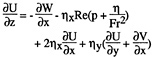
(17)

(18)
For the physical domain, the terminology normal and tangential refers to the mean free surface [i.e., (2)–(4) are the components of the stress in each of the Cartesian coordinate directions (z,x,y), respectively, on z=η]; however, upon transformation into the computational domain, it refers to the actual free surface z=η. Finally, (5) is solved for Wz to provide the free-surface boundary condition for W
(19)
Equations (16)–(19) were implemented in finite-difference form using backward differences for the z-derivatives and central differences for the x-and y-derivatives, for (16) and (19) and a backward and central differences, respectively, for the x- and y-derivatives for (17) and vice versa for (18).
For turbulent flow,
(20)
However, the same conditions (16)–(19) apply for turbulent flow with V interpreted as the mean velocity. The kinematic free-surface boundary condition in terms of velocity fluctuations is
−u ηx−v ηy+w=0 (21)
Multiplying (21) by u, v, and w and Reynolds averaging results in, respectively
(22)
(23)
(24)
Substituting (20) into (14) and using (22)–(24) to eliminate the Reynolds-stress terms results identically in (16)–(18), but with V interpreted as the mean velocity. Note that this derivation neglects the effects of free-surface fluctuations. Equation (19) is also valid for the mean-velocity components. The finite-difference procedures for turbulent flow were the same as those described earlier for laminar flow.
Reasonable approximations for free-surface boundary conditions for k and ε are simply zero-gradient conditions
(25)
(26)
on z=η, which are implemented in finite-difference form using backward differences for the z-derivatives.
In summary, for laminar flow, the exact free-surface boundary conditions are given by (13) and (16)–(19). The corresponding turbulent-flow approximation are these same conditions and (25)–(26). Approximate treatments of the free-surface boundary conditions are now considered, which are useful in assessing various approximations used in the precursory and relevant work, i.e., flat free-surface, inviscid, and zero-gradient conditions.
The flat free-surface conditions are obtained from the exact conditions under the approximation that ηx=ηy=0 in the dynamic free-surface boundary conditions, whereupon (16) –(18) reduce to
(27)
(28)
(29)
The inviscid conditions are obtained from the flat free-surface conditions under the additional assumption that the normal and tangential gradients of the normal velocity are negligible, whereupon (27)–(29) reduce to
(30)
(31)
(32)
(27–(29) and (30)–(32) in conjunction with (13) and (19) are solved in a similar manner as described earlier for the exact conditions, including, for turbulent flow, (25)–(26). The zero-gradient conditions are obtained from the inviscid conditions under the additional assumption that (30) and (19) are replaced by zero-gradient conditions
(33)
(34)
which in conjunction with (31)–(32) are solved in a similar manner as described earlier for the exact conditions, including, for turbulent flow, (25)– (26); however, in this case, (13) is not required since η is no longer present in the equations.
The exact and approximate free-surface boundary conditions are to be applied on the exact free-surface z=η, which is obtained as part of the solution. However, with the additional assumption that the wave elevation is small, all of the above conditions can be represented by first-order Taylor series expansions about the mean wave-elevation surface (i.e., z=0). In the following, this will be referred to as the Taylor-series approximation.
COMPUTATIONAL CONDITIONS, GRIDS, AND UNCERTAINTY
The computational conditions were based on [1–3], i.e., Ak=(0, .01, .11, .21), Re=105 and 1.64×10⁶ for laminar2 and turbulent flow, respectively, and L=λ=1. Typical values for δb (at the trailing edge), δw (in the near wake), and δfs (at the edge of the blw) are (.015, .02, .0018) and (.02, .03, .0004) for laminar and turbulent
flow, respectively. The corresponding Ak/ε values for both laminar and turbulent flow are O(1) and O(10) for small and medium and large steepness, respectively.
The laminar-flow calculations were performed for all four Ak values utilizing the exact, flat free-surface, inviscid, and zero-gradient conditions applied both on z=η (exact) and 0 (Taylor-series approximation). For zero steepness, the calculations were begun with a zero-pressure initial condition for the pressure field. For nonzero steepness, the complete zero-steepness solution was used as an initial condition. The solutions were built up in stages starting with small Ak values and achieving partial convergence and then incrementally increasing Ak until reaching the desired value and final convergence. For each Ak>0, initially coarse-grid calculations were performed utilizing the zero-gradient condition applied on z=0. These were then used as the initial guess for the fine-grid calculations utilizing the exact and approximate conditions applied both on z=0 and η. For the cases involving free-surface conforming grids (i.e., conditions applied on z= η), usually three updates (i.e., grid regenerations) were sufficient for convergence. Partial views of the coarse and typical fine grids used in the calculations are shown in figure 4. For the coarse grid, 170 axial, with 50 over the plate and 120 over the wake, 24 transverse, and 9 depthwise grid points were used, i.e., imax was 170×24×9 =36720. For the fine grid, 179 axial, with 5 before the leading edge, 54 over the plate and 120 over the wake, 24 transverse, and 25–27 depthwise, with 16–18 over the free-surface boundary layer, grid points were used, i.e., imax was 179×24×27=115992.
The turbulent-flow calculations were performed for all four Ak values utilizing the zero-gradient conditions applied on z=0 and, for Ak=.01, utilizing the exact and zero-gradient conditions on z=η and 0. The procedure for obtaining the solutions was similar to that for laminar flow. Transition was fixed at x=.05, which corresponds to the turbulence stimulators in the experiments. For the coarse grid, 187 axial, with 49 over the plate and 138 over the wake, 24 transverse, with 15 in the inner layer, and 9 depthwise grid points were used, i.e., imax was 187×24×9=40392. The fine grid was similar, except 28 depthwise, with 12 over the free-surface boundary layer, grid points were used, i.e., imax was 187×24×28=125664.
The detailed grid information, and values of the time, velocity, pressure-correction, and pressure under-relaxation factors and total number of global iterations itl used in obtaining both the laminar and turbulent solutions are provided in [8]. The average job run CRAY hours and central memory were 1.05 and 1.17 hours and 1.5 megawords for 100 global iterations for the fine-grid laminar and turbulent solutions, respectively.
Due to the complexity of the present calculations, it was not possible to carry out extensive grid dependency and convergence tests; however, these were done previously both for the basic viscous-flow method [11] and for other applications. The convergence criterion was based on the residual
(35)
and error(x,y,z) in satisfying the dynamic free-surface boundary conditions (17), (18), and (16), respectively, i.e., that R(it) and the error (x,y,z) be of order 10−4. Typical convergence histories and error-bar charts are provided in [8] and figure 5, respectively.
LAMINAR-FLOW SOLUTIONS
First, the small wave-steepness Ak=.01 results are discussed in detail for both the macro and micro scales: the macro scale corresponds to λ=L=1 and includes region III, whereas the micro scale corresponds to the body blw and free-surface boundary-layer thicknesses and is restricted to region IV. Second, the medium and large wave-steepness Ak=.11 and .21 results are discussed with particular reference to the influences of increasing Ak, including wave-induced separation. In general, only detailed results are presented in which the exact free-surface boundary conditions were utilized; however, in the discussion of the error-bar charts, reference is made to the various approximate treatments discussed earlier.
The discussion focuses on the differences between the Ak=0 or equivalently deep solutions and the nonzero wave-steepness Ak=.01, .11, and .21 solutions through the presentation of dependent variable differences from their deep values
Δ![]() =
=![]() −
−![]() (deep) (36)
(deep) (36)
where ![]() is any of the relevant dependent variables of interest, e.g., V, p, ω, etc.; thereby, accentuating the wave-induced effects. The equivalence between the Ak=0 and deep solutions is indicated by the form of the governing equations and free-surface boundary conditions with η=ηx=ηy=W=0 (except for small leading- and trailing-edge effects for the
is any of the relevant dependent variables of interest, e.g., V, p, ω, etc.; thereby, accentuating the wave-induced effects. The equivalence between the Ak=0 and deep solutions is indicated by the form of the governing equations and free-surface boundary conditions with η=ηx=ηy=W=0 (except for small leading- and trailing-edge effects for the
former case, which were neglected since only zero-gradient conditions were used). Furthermore, note that both the Ak=0 and deep solutions correspond to the Blasius solution and corresponding two-dimensional wake, both of which are recovered to within a few percent, except for leading- and trailing-edge and near-wake effects. In general, results are presented and/or discussed for both the blw and fw regions.
In order to confirm the ome for regions III and IV and for evaluation of the relative contributions of various terms in the equations of interest, average values over the blw thickness are evaluated and designated with an overbar
(37)
where, in this case, ![]() is any relevant dependent variable or equation, i.e., (13b), (16) –(19), and the vorticity difference, vorticity-transport equation, and free-surface vorticity flux, respectively
is any relevant dependent variable or equation, i.e., (13b), (16) –(19), and the vorticity difference, vorticity-transport equation, and free-surface vorticity flux, respectively
(38)

(39a)
(39b)

39c)
(40a)
(40b)
(40c)
Figures for ![]() are included where appropriate in which the numbered dashed and solid lines designated on the figures correspond to the various terms in the equations with the numbering proceeding term by term from left to right. In most cases, the dashed line corresponds to the term representing the left-hand side of the equation. In the cases of (16)–(18) and the vorticity-transport equation, the dashed line represents the sum of all the terms, which, of course, should be zero. In discussing such figures,
are included where appropriate in which the numbered dashed and solid lines designated on the figures correspond to the various terms in the equations with the numbering proceeding term by term from left to right. In most cases, the dashed line corresponds to the term representing the left-hand side of the equation. In the cases of (16)–(18) and the vorticity-transport equation, the dashed line represents the sum of all the terms, which, of course, should be zero. In discussing such figures, ![]() is identified in symbol with an overbar or in words with inclusive terms simply referred to in symbol without an overbar or by number. Note that the solutions are for the primitive variables V and p subject to the free-surface boundary conditions (13b) and (16) –(19), whereas equations (38)–(40) are derived, which in conjunction with the integration procedure (37) introduces some error; however,
is identified in symbol with an overbar or in words with inclusive terms simply referred to in symbol without an overbar or by number. Note that the solutions are for the primitive variables V and p subject to the free-surface boundary conditions (13b) and (16) –(19), whereas equations (38)–(40) are derived, which in conjunction with the integration procedure (37) introduces some error; however, ![]() are still useful in evaluating the solutions.
are still useful in evaluating the solutions. ![]() are evaluated at z= .1 and η for the macro- and micro-scale flows, respectively. Appendix B in [8] provides a summary of the ome for the various variables or equations of interest, including a listing of the confirmations and exceptions based on the blw averaged values.
are evaluated at z= .1 and η for the macro- and micro-scale flows, respectively. Appendix B in [8] provides a summary of the ome for the various variables or equations of interest, including a listing of the confirmations and exceptions based on the blw averaged values.
Lastly with regard to the presentation of the results, the analysis was facilitated by color graphics through the use of PLOT3D from which certain of the present figures were reproduced in black and white. Note that in such figures—W is shown in conformity with the PLOT3D coordinate system (figure 3), i.e., negative values correspond to downward flow and positive values to upward flow.
Small Steepness
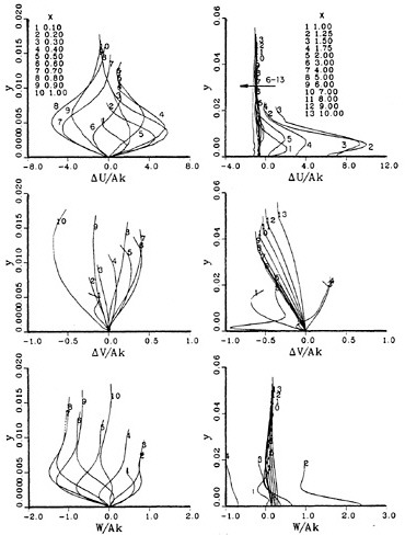
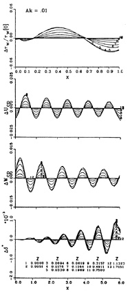
First, the results for the macro-scale flow are discussed. Figure 6 displays the free-surface velocity profiles ΔV/Ak vs. y for various axial locations. The streamwise ΔU and depthwise ΔW components display the pressure-gradient induced acceleration and deceleration phases and alternating direction, respectively. The transverse component ΔV indicates outward flow over most of the plate and inward flow near the trailing edge and over most of the wake. Note that the ome conform to table 1, i.e., V=(1,ε,Ak) and (1,ε/x,Ak) for the blw and fw, respectively. Also, noteworthy for laminar flow, is the broad region of large velocity gradients over δ. The results at larger depths are qualitatively similar, but with reduced amplitudes due to the exponential depthwise decay of the streamwise pex and depthwise pez external-flow pressure gradients.
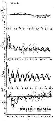
Figure 7 displays the wall-shear stress ![]() wake-centerplane velocities ΔUcp and ΔVcp, and displacement thickness Δδ* vs. x for various depthwise locations. The wave-induced oscillations are evident as is the wake bias. The oscillations persist to large depths, i.e.,
wake-centerplane velocities ΔUcp and ΔVcp, and displacement thickness Δδ* vs. x for various depthwise locations. The wave-induced oscillations are evident as is the wake bias. The oscillations persist to large depths, i.e.,
wave effects are discernible up to about z=.5; however, the largest variations are near the free surface and, subsequently, decay rapidly towards the deep solution. The amplitudes of the oscillations are large, especially in the near and intermediate wake. The large values of Δδ* near the trailing edge are associated with wave-induced separation, which occurs in this region for sufficiently large Ak. The wake bias [8] refers to the fact that the flow in the near and intermediate wake is considerably more responsive to the effects of the favorable as compared to the adverse external-flow pressure gradients, i.e., the magnitude of the overshoots in response to favorable pex and pez are much larger than those in response to adverse pex and pez. Subsequently, there is transition region where the differences between the maximum and minimum amplitudes decay such that ultimately in the fw (x![]() a periodic state is recovered in which ΔUcp, ΔWcp, and Δδ* all appear to oscillate with equal maximum and minimum amplitudes about the deep (i.e., two-dimensional) solution with, in some cases, a constant offset due to the wave-induced streaming velocities [ 8]. In the former cases, the ome of the oscillations is (Ak), which conforms to table 1. These trends are evident at all depths, but with reduced amplitudes. The distances over which the bias and transition occurs and magnitude of the streaming velocities depends on Ak and laminar- vs. turbulent-flow conditions, i.e., the bias and streaming velocity magnitude and extent are largest for small Ak and laminar flow.
a periodic state is recovered in which ΔUcp, ΔWcp, and Δδ* all appear to oscillate with equal maximum and minimum amplitudes about the deep (i.e., two-dimensional) solution with, in some cases, a constant offset due to the wave-induced streaming velocities [ 8]. In the former cases, the ome of the oscillations is (Ak), which conforms to table 1. These trends are evident at all depths, but with reduced amplitudes. The distances over which the bias and transition occurs and magnitude of the streaming velocities depends on Ak and laminar- vs. turbulent-flow conditions, i.e., the bias and streaming velocity magnitude and extent are largest for small Ak and laminar flow.
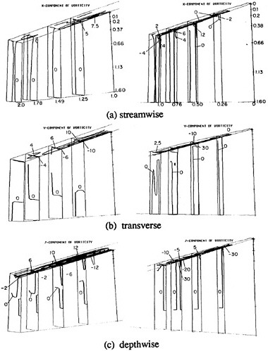
Figures 8 and 9 display ΔV and Δω contours, respectively, and vividly display the macro-scale wave-induced effects: acceleration and deceleration of the streamwise velocity component; alternating direction of the depthwise component (e.g., in the boundary-layer region, strong downward flow near x=.25, the indication of S-shaped profiles near x=.5 and 1, and strong upward flow near x=.75); depthwise decay of wave-induced effects; increased response, which propagates to larger depths, for the near- and intermediate-wake regions, including wake bias; and significant streamwise- and depthwise-vorticity components. Note the vertical scale and that the wave-induced effects persist to about z= .5. The blw averaged values of the vorticity components indicate that ω=(Wy,Uz−Wx,−Uy), which conforms to the table 1 ome (Ak/ε,1,1/ε) and ![]() for the blw and fw, respectively, with the exception of the −Wx term for the blw, which the ome indicates O(Ak).
for the blw and fw, respectively, with the exception of the −Wx term for the blw, which the ome indicates O(Ak).
Lastly, with regard to the Ak=.01 macro-scale solution, the results for the contours and blw averaged values of the convection (terms 1–3), stretching (terms 4–6, i.e., combined stretching/turning unless stated otherwise), and diffusion (term 7) terms of the streamwise, transverse, and depthwise vorticity-transport equations, respectively, are discussed. The contours for streamwise and stretching terms of the depthwise equation display the wavy nature of the flow, whereas the contours for the transverse equation and for the convective and diffusion terms of the depthwise equation are nearly zero and constant with depth, respectively. In the case of the streamwise equation, this is consistent with the nature of ωx (=Wy) itself, whereas in the case of the depthwise equation, this is consistent with the dominant stretching (and turning) terms, i.e., ωyWy+ωzWz and the nature of Wy and Wz. The blw averaged values indicate that for the blw, the streamwise, transverse, and depthwise equations primarily represent balances between, respectively: convection, stretching, and diffusion terms 1, 2, 4, 5, 6, and 7; convection, stretching, and diffusion terms 1, 2, 5, 6, and 7; and convection and diffusion terms 1, 2, and 7. Similarly for the fw, the streamwise, transverse, and depthwise equations primarily represent balances between, respectively: convection and diffusion terms 1 and 7; convection, stretching, and diffusion terms 1, 3, 6, and 7; and convection and diffusion terms 1 and 7. For each equation, in most cases, the dominant terms conform to the table 1 ome, i.e., respectively, for the blw (Ak/ε,1,ε−1) and for the fw [Ak/(εx3/2),Ak/x2,Ak/(εx3/2)]. The exceptions to the ome are for the ωx term ωxUx= (Ak/ε) for the blw, which the results indicate higher order; and the ωx and ωy terms ωyUy= (Ak2/εx3/2) and Wωyz=(Ak/x)2 and ωzVz= (Ak/x5/2), respectively, for the fw, which the results indicate lower order. Note that for the blw deep solution the only component of vorticity is ωz=−Uy=(ε−1), such that the streamwise and depthwise vorticity equations are identically zero and the depthwise equation is an exact balance between convection and diffusion terms 1 and 7 with ome (ε−1).
Based on the results for the vorticity-transport equation and associated ome and vorticity production ω(y=0)=(−Uy,0,Wy) and flux qw=(−Repz,0,Repx) on the plate, the nature
of the vorticity transport in region III is as follows. For the blw: ωz is produced/fluxed on the plate due to ωz(y=0) and qwz, respectively, and transported by a balance of convection and diffusion terms 1, 2, and 7 (=ωzyy); ωy is created by turning term 6 (=ωzVz) and transported by a balance of convection, stretching, and diffusion terms 1, 2, 5, and 7 (= ωyyy); and ωx is produced/fluxed on the plate due to ωx(y=0) and qwx, respectively, and created by turning terms 5 and 6 (=ωyUy+ ωzUz) and transported by a balance of convection and diffusion terms 1, 2, and 7 (=ωxyy). For the fw: ωx and ωz are transported by a balance of convection and diffusion terms 1 and 7 (=ωxyy and ωzyy, respectively), whereas ωy is created by turning term 6 (=ωzVz) and transported by a balance of convection and diffusion terms 1 and 7 (ωyyy).
Next, the results for the micro-scale flow are discussed. The differences between the exact and various approximate treatments of the free-surface boundary conditions are displayed in the error-bar chart for the dynamic free-surface boundary condition (figure 5). First, consider the results utilizing the Taylor-series approximation. The zero-gradient conditions lead to appreciable errors for all three stress components. The inviscid conditions reduce the errors substantially (i.e., by two orders of magnitude) and somewhat for the normal and transverse components, respectively, and have minimal effect on the streamwise component. The flat free-surface conditions have errors similar to those just described. The exact conditions substantially reduce the error for the streamwise component (i.e., by one order of magnitude) and somewhat for the normal and transverse components. The results utilizing the exact free surface are similar to those just described for the approximate treatments, i.e., have a minimal influence; however, for the exact conditions the errors for all three components are somewhat reduced. In summary, for small Ak=.01, the zero-gradient conditions lead to substantial errors, the inviscid and flat free-surface conditions reduce the error for the normal component, and the exact conditions additionally reduce the error for the streamwise and transverse components. Application of the conditions on the exact free surface has a minimal influence, except for the exact condition, which displays a slight reduction in error for all three components. Note that appreciable errors in satisfaction of the exact conditions correspond to the generation of erroneous vorticity near the free surface.
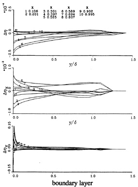
Figure 10a displays the solution of the kinematic free-surface boundary condition (13b) for the wave-elevation Δη and slopes Δηx and Δηy calculated using finite differences. The former are seen to correlate with W and the latter with—W in the blw and W in the fw, which, at least in magnitude, is expected both from physical reasoning and the form of (13). In the fw ![]() , Δη monotonically decreases in amplitude such that Δηx → Δηy → 0. Figure 10b shows
, Δη monotonically decreases in amplitude such that Δηx → Δηy → 0. Figure 10b shows ![]() and
and ![]() evaluated both using (13b) and finite differences. The dominant terms for the blw are, respectively, W/U and −ηXU/V, whereas for the fw, in the latter case, the dominant term is W/V. η, ηx, and ηy conform to the expected ome, i.e., for the blw and fw (Ak,Ak,Ak/ε) and(Ak,Ak,Ak), respectively.
evaluated both using (13b) and finite differences. The dominant terms for the blw are, respectively, W/U and −ηXU/V, whereas for the fw, in the latter case, the dominant term is W/V. η, ηx, and ηy conform to the expected ome, i.e., for the blw and fw (Ak,Ak,Ak/ε) and(Ak,Ak,Ak), respectively.
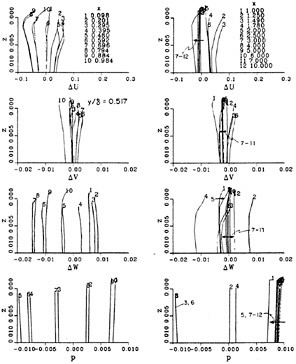
Figures 11a-d display ΔV contours and the blw averaged values of the dynamic and continuity-equation free-surface boundary conditions ![]() , and
, and ![]() evaluated using (17)–(19), and (16), respectively. The ΔU and ΔV contours display large variations, including islands of large magnitudes, whereas those for ΔW and Δp indicate relatively smooth variations. Note the vertical scale and that the effects of the free-surface boundary conditions penetrate to a depth of about z≈.04 (≈λ/25≈3δb). The table 1 ome are confirmed, i.e.: for the blw, the dominant terms are ηyUy (−Wy+2ηyVy+ηxUy),−(Ux+ Vy), and −η/Fr2 with ome (Ak/ε2,Ak/ε,1,Ak/Fr2), respectively, whereas for the fw, the dominant terms are −Wx, −Wy, −(Ux+Vy), and −η/Fr2 with ome
evaluated using (17)–(19), and (16), respectively. The ΔU and ΔV contours display large variations, including islands of large magnitudes, whereas those for ΔW and Δp indicate relatively smooth variations. Note the vertical scale and that the effects of the free-surface boundary conditions penetrate to a depth of about z≈.04 (≈λ/25≈3δb). The table 1 ome are confirmed, i.e.: for the blw, the dominant terms are ηyUy (−Wy+2ηyVy+ηxUy),−(Ux+ Vy), and −η/Fr2 with ome (Ak/ε2,Ak/ε,1,Ak/Fr2), respectively, whereas for the fw, the dominant terms are −Wx, −Wy, −(Ux+Vy), and −η/Fr2 with ome ![]() , respectively. The exception to the ome is for the Vz term 2ηyVy=(Ak/ε) for the blw, which the results indicate higher order. The trends for
, respectively. The exception to the ome is for the Vz term 2ηyVy=(Ak/ε) for the blw, which the results indicate higher order. The trends for ![]() follow ηyUy such that regions of Uz > and <0 imply ΔU near the free surface is smaller and larger than at greater depths, respectively, which is also the case for the other velocity components ΔV and ΔW and their derivatives Vz and Wz. In the blw, this is achieved in a remarkable manner, i.e., the maximum/minimum values are below the free surface: in regions of Uz<0, there is an island of large negative ΔU below the free surface, whereas in regions of Uz >0, there is an island of large positive ΔU below the free surface. For
follow ηyUy such that regions of Uz > and <0 imply ΔU near the free surface is smaller and larger than at greater depths, respectively, which is also the case for the other velocity components ΔV and ΔW and their derivatives Vz and Wz. In the blw, this is achieved in a remarkable manner, i.e., the maximum/minimum values are below the free surface: in regions of Uz<0, there is an island of large negative ΔU below the free surface, whereas in regions of Uz >0, there is an island of large positive ΔU below the free surface. For ![]() , Uz becomes small, i.e., follows—Wx. The Vz trends are complex since all three terms-Wy, ηxUy, and 2ηyVy contribute, although the latter term is of relatively smaller magnitude. In the blw, ΔV also displays islands of large positive/negative values below the free surface.
, Uz becomes small, i.e., follows—Wx. The Vz trends are complex since all three terms-Wy, ηxUy, and 2ηyVy contribute, although the latter term is of relatively smaller magnitude. In the blw, ΔV also displays islands of large positive/negative values below the free surface.
In the near and intermediate wake, Vz >0 such that ΔV is smaller near the free surface than at greater depths, but with the minimum value at the free surface itself. For x![]() , Vz becomes small, i.e., follows—Wy. The trends for
, Vz becomes small, i.e., follows—Wy. The trends for ![]() follow– (Ux+Vy). In the blw, Wz is small such that the variations are also small, except near the trailing edge and in the near and intermediate wake where Wz<0, including islands of minimum values below the free surface. For x
follow– (Ux+Vy). In the blw, Wz is small such that the variations are also small, except near the trailing edge and in the near and intermediate wake where Wz<0, including islands of minimum values below the free surface. For x![]() , Wz becomes relatively smaller, i.e., follows—(Ux+Vy). The p̅ trends follow—η. The depthwise variations of velocity and pressure are further displayed in figure 12 in which ΔV and p vs. z at y/δ=.52 are shown. Maximum/minimum values below the free surface are evident for all three velocity components, whereas p is nearly uniform.
, Wz becomes relatively smaller, i.e., follows—(Ux+Vy). The p̅ trends follow—η. The depthwise variations of velocity and pressure are further displayed in figure 12 in which ΔV and p vs. z at y/δ=.52 are shown. Maximum/minimum values below the free surface are evident for all three velocity components, whereas p is nearly uniform.
Figures 13a-d display Δω contours and the blw averaged values ![]()
![]() .
.
All three components display large variations near the free surface and islands of maximum/minimum values, especially ωy. The dominant terms for the blw are 2Wy−ηxUy, ηyUy, and Uy, which conform to the table 1 ome (Ak/ε,Ak/ε2,1/ε), respectively; however, the ome also indicate that the ωx term—2ηyVy=(Ak/ε), but the results indicate higher order. The dominant terms for the fw are Wy−Vz,−Wx, and −Uy, which conform to the table 1 ome ![]() respectively; however, the ome also indicate that the ωy term Uz=(Ak/x), but the results indicate higher order. Noteworthy are the large values of transverse vorticity ωy for the blw, which are a direct consequence of the free-surface boundary conditions. For x
respectively; however, the ome also indicate that the ωy term Uz=(Ak/x), but the results indicate higher order. Noteworthy are the large values of transverse vorticity ωy for the blw, which are a direct consequence of the free-surface boundary conditions. For x![]() , all three vorticity components are negligible. The depthwise variations of vorticity at y/δ=.52 indicate maximum/minimum values below the free surface for all three vorticity components. The fact that the velocity and vorticity components display maximum/minimum values below the free surface is similar and consistent with the oscillatory nature of the viscous Stokes-wave solution for region II (cf. figure 96 of [8]).
, all three vorticity components are negligible. The depthwise variations of vorticity at y/δ=.52 indicate maximum/minimum values below the free surface for all three vorticity components. The fact that the velocity and vorticity components display maximum/minimum values below the free surface is similar and consistent with the oscillatory nature of the viscous Stokes-wave solution for region II (cf. figure 96 of [8]).
The results for the streamwise, transverse, and depthwise vorticity flux both on the free surface (40) and plate are now discussed, including, in the former case, the blw averaged values. Note that q and qw >0 correspond to vorticity flux out and into the fluid, respectively. On the free surface, the dominant terms for the blw are −ηyωxy, −ηyωyy, and −ηyωzy+ωzz, which conform to the table 1 ome (Ak/ε2, Ak/ε3, 1/ε2), respectively; however, the ome also indicate that the (qx,qy) terms (ωxz,ωyz)= (Ak/ε2,Ak/ε3), but the results indicate higher order. The dominant terms for the fw are − ηyωxy, −ηyωyy, and −ηyωZy, which conform to the table 1 ome [Ak2/(ε2x), Ak2/(εx3/2), Ak2/ε2x)], respectively; however, the streamwise vorticity-flux terms −ηyωxy=(Ak2/ε2x) and ωxz =(Ak/εx3/2), but the results indicate higher and lower order, respectively; and the depthwise vorticity-flux terms −ηyωZy=(Ak2/ε2x) and ωzz =(Ak/εx3/2), but the results indicate higher and lower order, respectively. For ![]() , all three vorticity-flux components are negligible. On the plate, the dominant terms are −ωxy=−Re pz, ωyy=0, and −ωzy=Re px with ome [Ak/(ε2Fr2)] in the former and latter cases. Note that q can also be expressed by vector identity as [12]
, all three vorticity-flux components are negligible. On the plate, the dominant terms are −ωxy=−Re pz, ωyy=0, and −ωzy=Re px with ome [Ak/(ε2Fr2)] in the former and latter cases. Note that q can also be expressed by vector identity as [12]
q=n×![]() ×ω−(
×ω−(![]() ω) · n (41)
ω) · n (41)
The terms on the right-hand side of (41) can be further expanded through the use of the NS equation and vector identity, respectively, to read
n×![]() ×ω=n×[−Re(a+
×ω=n×[−Re(a+![]() p)] (42)
p)] (42)
(![]() ω) · n=
ω) · n=![]() (ω · n)−ω ·
(ω · n)−ω · ![]() n (43)
n (43)
where a is the acceleration. (42) is a vector tangent to the free surface with magnitude proportional to the sum of the acceleration and piezometric pressure gradient. (43) is the sum of the gradient of the normal component of vorticity and dot product of ω and ![]() n, which is related to the surface curvature. Thus, the physical mechanism for q is a combination of these terms. Expansion of (41) and comparison with (40a)– (40c) shows that terms 2, 3, and 4 correspond to [(43), (42), (42)], [(42), (43), (42)], and [(42), (42), (43)], respectively. Lastly, the ome of the momentum equations at the free surface indicate for the blw and fw, respectively
n, which is related to the surface curvature. Thus, the physical mechanism for q is a combination of these terms. Expansion of (41) and comparison with (40a)– (40c) shows that terms 2, 3, and 4 correspond to [(43), (42), (42)], [(42), (43), (42)], and [(42), (42), (43)], respectively. Lastly, the ome of the momentum equations at the free surface indicate for the blw and fw, respectively
WUZ=−Re−1(−ωyz)=(Ak/ε)2
WVz=−Re−1(ωxz)=(Ak2/ε)
UWx+VWy+WWz−Pz=
−Re−1(ωyx−ωxy)=(Ak) (44a)
and
UUx=−Re−1(ωzy)=(Ak/x)
UVx=−Re−1(ωxz−ωzx)=(ε/x2) (44b)
UWx=−Re−1(ωxy)=(Ak/x)
which relate certain q terms [i.e., right-hand sides of (44)] to certain terms of the tangential and normal components of the acceleration and piezometric pressure gradient on the free surface [i.e., left-hand sides of (44)].
Lastly, with regard to the Ak=.01 micro-scale flow, the results for the vorticity-transport equation are discussed. The contours for all three equations and terms display significant variations with depth, especially for the transverse equations. The blw averaged values indicate that for the blw the streamwise, transverse, and depthwise equations primarily represent balances between, respectively: stretching terms 5 and 6; convection and diffusion terms 3 and 7; and convection, stretching, and diffusion terms 1, 2, 6, and 7. In the former case, the balance is actually between convection, stretching, and diffusion terms 1, 2, 4, 5, 6, and 7 (=ωxyy) with ome (Ak/ε) or convection and diffusion terms 3 and 7 (=ωxzz) with ome (Ak/ε)3; since, ωyUy+ωzUz =−WxUy+VxUz=(Ak/ε) due to the cancellation of the UzUy=(Ak/ε3) terms. Similarly for the fw, the streamwise, transverse, and depthwise equations primarily represent balances between: convection and diffusion terms 1 and 7. For each equation, in most cases, the dominant terms conform to the table 1 ome, i.e., respectively, for the blw [Ak/ε or (Ak/ε)3, Ak3/ε4,ε−1] and for the fw [Ak/(εx3/2),Ak/x2,Ak/(εx3/2)]. The exceptions to the ome are for the ωx terms Vωxy=(Ak/εx2) and Wωxz=ωxUx=ωyUy=ωzUz= (Ak2/εx3/2) for the fw, which the results indicate lower order. Consistent with ω, all three equations indicate negligible values for x![]() .
.
Based on the results for the vorticity-transport equation and associated ome, vorticity production ω(y=0) on the plate and flux both on the plate qw and free surface q the nature of the vorticity transport in region IV is as follows. For the blw: ωz is produced/fluxed on the plate due to ωz(y=0) and both on the plate and free surface due to qwz and qz, respectively, and transported by a balance of convection, stretching, and diffusion terms 1, 2, 6, and 7 (= ωzyy); ωy is fluxed on the free surface due to qy and transported by a balance of convection and diffusion terms 3 and 7 (=ωyzz); and ωx is produced/fluxed on the plate due to ωx(y=0) and both on the plate and free surface due to qwx and qx, respectively, and created by turning terms 5 and 6 (=ωyUy+ωzUz) and transported by a balance of convection, stretching, and diffusion terms 1, 2, 4, 5, 6, and 7 (=ωxyy) or convection and diffusion terms 3 and 7 (=ωxzz). For the fw: ω is fluxed on the free surface due to q and transported by a balance of convection and diffusion terms 1 and 7.
Medium and Large Steepness
The trends for the medium- and large-steepness macro-scale flow are similar to those described earlier for small steepness, with the exception of the influences of wave-induced separation. The wave-induced separation flow patterns for both Ak=.11 and .21 are nearly identical with those obtained previously [3] in which the zero-gradient approximation was utilized for the free-surface boundary conditions, although the effects of the free-surface boundary conditions cause a small increase in the size of the separation region. Also evident is that the wave-induced effects when normalized by Ak are larger forAk=.01.
The trends for the micro-scale flow are also similar to those described earlier for Ak= .01, except the following: there is an increased influence of satisfying the free-surface boundary conditions on the exact free-surface z=η; the wave elevation and slopes show complex behavior in the separation region, especially for Ak=.21; the depthwise velocity and pressure profiles indicate that the ΔU variations are reduced, whereas those for ΔV, ΔW, and Δp are increased; and the variations are confined to a narrower region close to the free surface. Also, in general, the table 1 ome are confirmed.
TURBULENT-FLOW SOLUTIONS
The small-wave steepness Ak=.01 results are discussed for both the macro and micro scales in which the turbulent-flow approximation to the exact free-surface boundary conditions is utilized, i.e., (13), (16)–(19), and (25–(26). Note that, as was the case for laminar flow, the Ak=0 and deep solutions are equivalent due, here again, to the use of the zero-gradient condition and, additionally, an isotropic eddy viscosity. Both the Ak=0 and deep solutions correspond to benchmark two-dimensional flat-plate boundary layer and wake turbulent-flow solutions within a few percent, except for leading- and trailing-edge and near-wake effects. In [8] results are also presented for Ak=.11 and .21 in which the zero-gradient approximation to the free-surface boundary conditions was utilized and
comparisons were made with the precursory data and calculations, which validated the performance of the two-layer k-ε model.
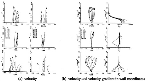
Figures 14 and 15 display ΔV/Ak and ΔVy vs. y and y+ and ![]() , ΔUcp, ΔWcp, and Δδ* vs. x, respectively. Comparison to the corresponding laminar-flow solutions indicates similar tendencies, although the influences of turbulence are clearly evident, i.e.: typical turbulent profiles with a narrow region of large velocity gradients very close to the wall and wake centerplane; reduction in overshoots, three-dimensionality, and wake bias and streaming velocities; and wave-induced separation is not present. The ΔVy profiles indicate that the region of large velocity gradient is confined to y+<10. As will be discussed next, this has direct consequences with regard to the micro-scale flow. In general, the table 1 ome are confirmed.
, ΔUcp, ΔWcp, and Δδ* vs. x, respectively. Comparison to the corresponding laminar-flow solutions indicates similar tendencies, although the influences of turbulence are clearly evident, i.e.: typical turbulent profiles with a narrow region of large velocity gradients very close to the wall and wake centerplane; reduction in overshoots, three-dimensionality, and wake bias and streaming velocities; and wave-induced separation is not present. The ΔVy profiles indicate that the region of large velocity gradient is confined to y+<10. As will be discussed next, this has direct consequences with regard to the micro-scale flow. In general, the table 1 ome are confirmed.
The results for the error-bar chart for turbulent flow (figure 5) indicate that the differences between the errors for the zero-gradient and turbulent-flow approximation to the exact free-surface boundary conditions are similar to those for laminar flow; however, it is also evident that the error has not been reduced to the same level. Figures 16–18 display, respectively, Δη, Δηx, Δηy, and ΔV and Δω contours. Comparison to the corresponding laminar-flow solutions indicate, as was the case for the macro-scale flow, similar tendencies, although, here again, the influences of turbulence are clearly evident, i.e., in this case, the effects of the free-surface boundary conditions are confined to a very narrow region close to the wall and free surface, which correlates with the region of large velocity gradients (y+<10). This should not be surprising in view of the similarities between the exact laminar-flow free-surface boundary conditions and those presently used for turbulent flow. However, this underscores the need for confirmation of appropriate turbulence free-surface boundary conditions and refined treatment of region V for turbulent-flow conditions. In general, the table 1 ome are confirmed.
SUMMARY AND CONCLUSIONS
Definitive results have been presented, which, for the first time, document the nature of the flow for a solid-fluid juncture blw with waves, including the role of the free-surface boundary conditions. Overviews of the physical problem, including ome, precursory and relevant work, and the computational method were given. The computational conditions, grids, and uncertainty were described and results presented for small, medium, and large wave-steepness for laminar and turbulent flow.
The laminar and turbulent macro-scale flow (i.e., at scales corresponding to the wave length λ=L=1) exhibits all of the features of the wave-induced effects described for the blw region in the precursory work. Additionally, the nature of the vorticity production/flux/transport is explicated. Furthermore, at this scale, the effects of the free-surface boundary conditions are not discernible, which is also consistent with the precursory work in which it was found that most of the results could be explicated in terms of the external-flow pressure gradients without consideration of the role of the free-surface boundary conditions.
The laminar micro-scale flow (i.e., at scales corresponding to the body blw and free-surface boundary-layer thicknesses) indicates that the free-surface boundary conditions have a profound influence on the flow in the region close to the free surface, i.e., ![]() (≈λ/25≈3δb). Appreciable errors are introduced through approximations to the exact free-surface boundary conditions, which corresponds to the generation of erroneous vorticity near the free surface. The blw wave elevation and streamwise and transverse slopes correlate with the depthwise velocity component. The streamwise and transverse velocity components and vorticity components display large variations, including islands of large magnitudes (i.e., maximum/minimum values), whereas the depthwise velocity component and pressure indicate relatively smooth variations. All three components of vorticity flux on the free surface indicate significant values. The vorticity-transport equations display complex balances between convection, stretching/turning, and diffusion. For
(≈λ/25≈3δb). Appreciable errors are introduced through approximations to the exact free-surface boundary conditions, which corresponds to the generation of erroneous vorticity near the free surface. The blw wave elevation and streamwise and transverse slopes correlate with the depthwise velocity component. The streamwise and transverse velocity components and vorticity components display large variations, including islands of large magnitudes (i.e., maximum/minimum values), whereas the depthwise velocity component and pressure indicate relatively smooth variations. All three components of vorticity flux on the free surface indicate significant values. The vorticity-transport equations display complex balances between convection, stretching/turning, and diffusion. For ![]() , the effects of the free-surface boundary conditions become negligible. The wave-induced effects when normalized by wave steepness are larger for small than for medium and large steepness with the exception of the large influence of wave-induced separation; however, the free-surface boundary conditions have a relatively small influence on this catastrophic event. In general, the ome are confirmed for both the blw and fw, which confirms the importance of the parameter Ak/ε for characterizing the micro-scale flow.
, the effects of the free-surface boundary conditions become negligible. The wave-induced effects when normalized by wave steepness are larger for small than for medium and large steepness with the exception of the large influence of wave-induced separation; however, the free-surface boundary conditions have a relatively small influence on this catastrophic event. In general, the ome are confirmed for both the blw and fw, which confirms the importance of the parameter Ak/ε for characterizing the micro-scale flow.
The turbulent micro-scale flow results are similar and consistent with those for laminar flow, but must be considered preliminary due to the present uncertainty in appropriate treatment of
the turbulence free-surface boundary conditions and meniscus boundary layer for this condition. Clearly, both these areas are imperative for future study. For this purpose, current work involves further towing-tank experiments using laser-doppler velocimeter measurements for the foil-plate model, including the region close to the free surface, and development of cfd methods, including moving contact-line boundary conditions and RaNS methods utilizing nonisotropic turbulence models and large-eddy and/or direct numerical simulations.
Lastly, the present work has several implications with regard to the practical application of ship blw's for nonzero Fr. In particular, the free-surface boundary conditions have been shown to have an important influence in regions of large velocity gradients and wave slopes, including significant free-surface vorticity flux and complex momentum and vorticity transport in a layer close to the free surface all of which scale with the parameter Ak/ε. Note that the present Ak/ ε values=O(1)–O(10) are similar to those for model and full-scale practical applications. Also, although turbulent-flow conditions prevail for practical applications, the boundary layer is relatively thick (in distinction from the present thin blw turbulent-flow condition), especially over the afterbody and wake, such that the region of influence of the free-surface boundary conditions is expected to be large over a significant portion of the blw (i.e., more similar to the present laminar- than turbulent-flow solutions), which will affect the detailed flow near the free surface, i.e., velocity, pressure, and vorticity values and gradients, bubble entrainment, and triggering of wave breaking and -induced separations, etc.; thereby, impacting the overall ship performance, including signatures and propeller-hull interaction. In conclusion, methods for calculating ship blw's for nonzero Fr (e.g., [6,7]) should be extended to include more exact free-surface boundary conditions and clearly it is all the more imperative that progress be made on both areas designated earlier for future work. It has been remarked that the most important layer of the ocean is the top millimeter, i.e., microlayer [13], which, at least for some multiple of this physical dimension, may also be the case for ship blw's.
ACKNOWLEDGMENTS
This research was sponsored by the Office of Naval Research under grant N00014–92-K-1092. The calculations were performed on the CRAY supercomputers of the Naval Oceanographic Office and National Aerodynamic Simulation Program. The derivation of the mean-velocity free-surface boundary conditions for turbulent flow was provided by Dr. K. Parthasarathy.
REFERENCES
1. Stern, F., “Effects of Waves on the Boundary Layer of a Surface-Piercing Body, ” J. of Ship Research, Vol. 30, No. 4, Dec. 1986, pp. 256–274.
2. Stern, F., Hwang, W.S., and Jaw, S.Y, “Effects of Waves on the Boundary Layer of a Surface-Piercing Flat Plate: Experiment and Theory,” J. of Ship Research, Vol. 33, No, 1, March, 1989, pp. 63–80.
3. Stern, F., Choi, J.E., and Hwang, W.S, “Effects of Waves on the Wake of a Surface-Piercing Flat Plate: Experiment and Theory,” J. of Ship Research, Vol. 37, No. 2, June 1993, pp. 102–118.
4. Toda, Y., Stern, F., and Longo, J., “Mean-Flow Measurements in the Boundary Layer and Wake and Wave Field of a Series 60 CB=0.6 Ship Model-Part 1: Froude Numbers 0.16 and 0.316,” J. of Ship Research, Vol. 36, No. 4, Dec. 1992, pp. 360–377.
5. Longo, J., Stern, F., and Toda, Y., “Mean-Flow Measurements in the Boundary Layer and Wake and Wave Field of a Series 60 CB=0.6 Ship Model-Part 2: Scale Effects on Near-Field Wave Patterns and Comparisons with Inviscid Theory,” J. of Ship Research, Vol. 37, No. 1, March, 1993, pp. 16–24.
6. Tahara, Y., Stern, F., and Rosen, B., “An interactive Approach for Calculating Ship Boundary Layers and Wakes for Nonzero Froude Number,” J. of Computational Physics, Vol. 98, No. 1, Jan, 1992, pp. 33–53.
7. Tahara, Y and Stern, F., “Validation of an Interactive Approach for Calculating Ship Boundary Layers and Wakes for Nonzero Froude Number,” to appear Computers and Fluids, 1994.
8. Choi, J.E., “Role of Free-Surface Boundary Layer Conditions and Nonlinearities in Wave/Boundary-Layer and Wake Interaction,” Ph.D. Thesis, The University of Iowa, Dec. 1993.
9. Schlichting, H., “Boundary-Layer Theory,” McGraw Hill Book Company, New York, 1979.
10. Chen, H.C. and Patel, V.C., “The How around Wing-Body Junctions,” Proc. Symposium on Numerical and Physical Aerodynamic Flows, Vol. 4, 1989.
11. Patel, V.C., Chen, H.C., and Ju, S., “Ship Stern and Wake Flow: Solutions and the Fully-Elliptic Reynolds-averaged Navier-Stokes
Equations and Comparisons with Experiments,” J. of Computational Physics, Vol. 88, June 1990, pp. 305–336.
12. Rood, E.P., “Interpreting Vortex Interactions With a Free Surface,” to appear J.of Fluids Engineering, 1994.
13. MacIntyre, F., “The Top Millimeter of the Ocean,” Scientific American, Vol. 230, No.5, 1974, pp. 62–77.
14. Newman, J.N., “Recent Research on Ship Waves,” Proc. 8th Symposium on Naval Hydrodynamics, Pasadena, CA, Aug. 1970, pp. 519–545.
Table 1. Order-of-magnitude estimates.
|
Region |
I |
II |
III |
IV |
fw: |
||
|
blw |
fw |
blw |
fw |
||||
|
U |
1 |
1 |
1 |
1 |
1 |
1 |
|
|
∂U |
Ak |
Ak |
1 |
Ak |
1 |
Ak |
|
|
V |
ε |
ε/x |
ε |
ε/x |
|||
|
W |
Ak |
Ak |
Ak |
Ak |
Ak |
Ak |
|
|
p |
Ak |
Ak |
Ak/Fr2 |
Ak/Fr2 |
|||
|
η |
Ak |
Ak |
Ak |
Ak |
|||
|
ηx |
Ak |
Ak |
Ak |
||||
|
ηy |
Ak/ε |
Ak |
|||||
|
∂/∂x |
1 |
1 |
1 |
1/x |
1 |
1/x |
|
|
∂/∂y |
1/ε |
|
1/ε |
|
|||
|
∂/∂z |
1 |
1 |
1 |
1/x |
1/x |
||
|
Uz |
Ak2 |
Ak2 |
1 |
Ak/x |
Ak/ε2 |
Ak/x |
4 |
|
Vz |
ε |
ε/x2 |
Ak/ε |
|
3 |
||
|
Wz |
Ak2 |
Ak2 |
Ak |
Ak/x |
1 |
Ak/x |
3 |
|
ωx |
Ak/ε |
|
Ak/ε |
|
3 |
||
|
ωy |
Ak2 |
1 |
Ak/x |
Ak/ε2 |
Ak/x |
3 |
|
|
ωz |
1/ε |
|
1/ε |
|
3 |
||
|
qx |
Ak/ε2 |
Ak2/(ε2x) |
3 |
||||
|
qy |
Ak/ε3 |
Ak2/(εx3/2) |
3 |
||||
|
qz |
1/ε2 |
Ak2/(ε2x) |
3 |
||||
|
vorticity-transport equation |
|||||||
|
stream wise |
Ak/ε |
Ak/(εx3/2) |
(Ak/ε)3 |
Ak/(εx3/2) |
3 |
||
|
transverse |
1 |
Ak/x2 |
Ak3/ε4 |
Ak/x2 |
3 |
||
|
depthwise |
1/ε |
Ak/(εx3/2) |
1/ε |
Ak/(εx3/2) |
3 |
||
|
Re |
1/ε2 |
1/ε2 |
1/ε2 |
1/ε2 |
1/ε2 |
||

Figure 1. Wave/boundary-layer and wake interaction [14].

Figure 2. Flow-field regions.
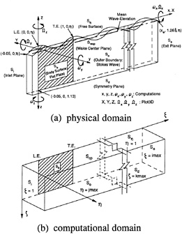
Figure 3. Stokes-wave/flat-plate flow field: solution domain and coordinate systems.

Figure 4. Laminar-flow computational grids.
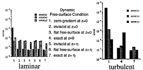
Figure 5. Error-bar chart: Ak=.01.


DISCUSSION
by Professor M.Tulin, University of California, Santa Barbara
How important are the intersection effects for the wave pattern, or wave resistance, and for the stern wake (propeller plane) pattern?
Author's Reply
We thank both the oral and written discussers of our paper for their pertinent remarks.
The free-surface boundary conditions have been shown to have an important influence in regions of large velocity gradients and wave slopes. For practical applications, the boundary layer is relatively thick, especially over the afterbody and wake, such that the region of influence of the free-surface boundary conditions is expected to be large over a significant portion of the blw, which will effect the detailed flow near the free surface, i.e., velocity, pressure, and vorticity values and gradients, bubble entrainment, and triggering of wave breaking and induced separations, etc.; thereby, impacting the overall ship performance, including signatures and propeller-hull interaction.
DISCUSSION
by Professor K.Mori, Hiroshima University, Japan.
Are the boundary conditions of (25) and (26) obtained from experimental data? According to our experiments [1], although the phenomena are not the same, the conditions seem too strong.
1. Mori, K. and Shin, M., Proc. of 17th Sym. on Naval Hydrodynamics ( 1989).
Author's Reply
The turbulence free-surface boundary conditions (25)–(26) are not based on experimental data, but rather seem reasonable approximations in view of the available turbulence/free-surface interaction experimental data for idealized geometries. As pointed out in the text, procurement of experimental data for more relevant geometries and determination of appropriate turbulence free-surface boundary conditions are imperative for future study.
Direct Numerical and Large-Eddy Simulations of Turbulent Free-Surface Flows
D.G.Dommermuth (Science Applications International Corporation, USA)
E.A.Novikov (University of California, San Diego, USA)
ABSTRACT
Direct numerical simulations and large-eddy simulations of free-surface turbulence are performed to investigate the turbulent structure near the free surface, the roughening of the surface, and the dissipation and scattering of waves by turbulence. Recent laboratory measurements that show tendency of two-dimensional turbulence at the free surface are not supported by the present numerical simulations. In the absence of waves, the surface disturbance (surface roughness) is directly proportional to the component of the pressure that is induced by the vortical portion of the subsurface flow. Simple formulas for predicting surface roughness, which include the effects of hydrostatics and capillarity, are provided. The scattering and dissipation rates of wave energy due to turbulence are the same order as laminar dissipation for a 5cm gravity-capillary wave at an moderate Froude number. Turbulent scattering and dissipation are dominated by the effects of parasitic capillary waves and surfactants. In the far wake of a ship the effects of turbulent scattering and dissipation are minimal.
NOMENCLATURE
|
Re: |
Reynolds number |
|
Rλ: |
Taylor Reynolds number |
|
Fr: |
Froude number |
|
We: |
Weber number |
|
ρ: |
Density |
|
σ: |
Surface tension |
|
g: |
Gravity |
|
ν: |
Kinematic viscosity |
|
(x,y,z): |
Cartesian coordinates |
|
t: |
Time |
|
ui: |
Total velocity field |
|
Ui: |
Rotational velocity field |
|
|
Potential field |
|
η: |
Free-surface elevation |
|
ni: |
Unit normal on free surface |
|
(u,ν,w): |
Total velocity components |
|
(U,V,W): |
Rotational velocity components |
|
Π: |
Total pressure |
|
P: |
Vortical component of pressure |
|
Pa: |
Atmospheric pressure |
|
C: |
Correlation coefficient |
|
Δ: |
Grid spacing |
|
|
: SGS stress tensor |
|
μ: |
Scattering or dissipation rate |
|
F: |
Filter operator |
1
INTRODUCTION
Direct numerical simulations (DNS) of ship wakes are very difficult. Based on Kolmogorov's scaling laws the work and storage requirements of a direct numerical simulation are proportional to Re3 and Re9/4 respectively, where Re is the Reynolds number. Doubling the Reynolds number leads to an order of magnitude increase in the amount of work that is necessary to compute a turbulent flow. So for a ship wake, where the Reynolds number is O(109) based on ship length and velocity, direct numerical simulations are impossible now and in the forseeable future.
Large-eddy simulations (LES) attempt to overcome this problem by directly computing the large-scale features of the flow and analytically modeling the small-scale features. The basic assumption of LES is that the small-scale motion is statistically more universal even though the large-scale motion may strongly depend on geometry, external forces, boundary conditions, and initial conditions. Successful implementations of LES methods include studies of homogeneous turbulence, turbulent channel flow, and weather prediction. Here, we use LES to perform preliminary studies of turbulent free-surface flows.
LES formulations decompose the velocity field into its resolvable and subgrid-scale (SGS) components. The effectiveness of a LES formulation depends on how well the SGS stresses are modeled. The SGS stresses are typically formulated in terms of a turbulent eddy viscosity. Smagorinsky's [36] method is the most widely used SGS model in large-eddy simulations, but as Moin [22] discusses there are several problems associated with this model including:
-
The optimal choice of the coefficient in the expression for the eddy viscosity depends on the type of flow;
-
The limiting behavior of the SGS model is not correct near walls or free surfaces;
-
The model is too dissipative in laminar flow regions; and
-
The model does not allow transfer of energy from small scales to large scales.
Attempts to alleviate these problems have not been very successful, but there has been some progress. For example, Schumann [34] modifys the behavior of the SGS stresses near walls. As a result, Schumann's simulations of turbulent channel flow agree with experiments slightly better than those of Deardorff [4] whose SGS stress formulation does not account for anisotropy.
Besides modifying the behavior of the SGS stresses near boundaries, another improvement to the Smagorinsky model is to use the resolved flow field to predict the subgrid scales. The basic idea is to extrapolate from the resolved flow the behavior of the SGS stresses. For example, Germano, et al [9], use extrapolation to predict the Smagorinsky coefficient. The effects of their model vanish in the case of laminar flow. Lilly [15] has recently proposed a modification to the extrapolation scheme that uses a least-squares technique to remove a source of singularity.
We use Germano's scheme with Lilly's modification to study free-surface turbulence. A Helmholtz formulation is used to decompose the flow field into potential and vortical fields [6], and an adjustment procedure is used to eliminate the generation of spurious high-frequency waves due to imbalances in the initial conditions [7]. Fully-nonlinear free-surface boundary conditions are satisfied on the exact position of the free surface, and a preconditioned multigrid solution scheme is used to solve the nonlinear elliptic boundary-value problems [8].
We provide the mathematical and numerical formulations of our LES and DNS capabilities in Sections 2–4. The performance of the LES and DNS capabilities is illustrated by several validation studies in Sections 5 & 6. We then use the DNS capability to investigate the turbulent structure near the free
surface, the roughening of the surface by turbulence, and the scattering and dissipation of surface waves by turbulence in Section 7.
2
MATHEMATICAL FORMULATION
2.1
Field Equations
Consider the unsteady incompressible flow of a Newtonian fluid under a free surface, and let ![]() represent the filtered three-dimensional velocity field as a function of time. Here, the overbar denotes the large-eddy filter. Applying Helmholtz's theorem gives
represent the filtered three-dimensional velocity field as a function of time. Here, the overbar denotes the large-eddy filter. Applying Helmholtz's theorem gives
(1)
where ![]() is a filtered velocity-potential which describes the irrotational flow and
is a filtered velocity-potential which describes the irrotational flow and ![]() is a filtered solenoidal-field which describes the vortical flow such that
is a filtered solenoidal-field which describes the vortical flow such that
(2)
(3)
Since ![]() satisfies Laplace's equation and the divergence of the rotational field
satisfies Laplace's equation and the divergence of the rotational field ![]() is chosen zero, the total velocity field
is chosen zero, the total velocity field ![]() conserves mass. Note that
conserves mass. Note that ![]() may contain a portion of the irrotational field depending on how the boundary conditions are defined.
may contain a portion of the irrotational field depending on how the boundary conditions are defined.
Based on this Helmholtz decomposition of the velocity field, define the total-pressure ![]() in terms of a vortical pressure
in terms of a vortical pressure ![]() and an irrotational pressure as follows:
and an irrotational pressure as follows:
(4)
Here, the velocity and pressure terms are respectively normalized by uc and ![]() , where uc is the characteristic velocity and ρ is the density.
, where uc is the characteristic velocity and ρ is the density. ![]() is the Froude number and ℓc is the characteristic length. The vertical coordinate z is positive upward, and the origin is located at the mean free surface. Substituting these decompositions (1 & 4) into the Navier-Stokes equations gives
is the Froude number and ℓc is the characteristic length. The vertical coordinate z is positive upward, and the origin is located at the mean free surface. Substituting these decompositions (1 & 4) into the Navier-Stokes equations gives

(5)
where Re=ucℓc/ν is the Reynolds number and ν is the kinematic viscosity. The SGS stress tensor is defined by
(6)
The divergence of the momentum equations (5) used in combination with the mass-conservation equations (2 & 3) can be used to derive a Poisson equation for the vortical pressure:
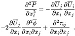
(7)
As shown by Dommermuth (1993a), the vortical pressure is also subject to a solvability condition because we impose Neumann boundary conditions [6].
2.2
Free-Surface Boundary Conditions
The Helmholtz decomposition of the velocity field requires that an additional boundary condition be imposed on the free surface. An expedient boundary condition that can be
specified is that the normal component of the rotational velocity is zero on the free surface:
(8)
where  is the filtered free-surface elevation and
 ![]() is the filtered unit-normal on the free surface. (The subgrid-scale terms in this equation and in the succeeding free-surface boundary conditions will be neglected.) The preceding constraint which is imposed on the rotational velocity field means that the evolution of the free-surface elevation is entirely prescribed in terms of the free-surface elevation itself and the velocity potential as follows:
is the filtered unit-normal on the free surface. (The subgrid-scale terms in this equation and in the succeeding free-surface boundary conditions will be neglected.) The preceding constraint which is imposed on the rotational velocity field means that the evolution of the free-surface elevation is entirely prescribed in terms of the free-surface elevation itself and the velocity potential as follows:
![]() , (9)
, (9)
where everything is evaluated on the exact position of the free surface, ![]()
The normal stress on the free surface must balance with the atmospheric pressure and the surface tension:
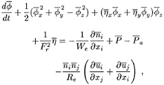
(10)
where ![]() is the atmospheric pressure, We=
is the atmospheric pressure, We= ![]() is the Weber number, and σ is the surface tension.
is the Weber number, and σ is the surface tension. ![]() is a substantial derivative. In addition to the normal-stress condition there are also two tangential-stress conditions that are provided in Dommermuth [6].
is a substantial derivative. In addition to the normal-stress condition there are also two tangential-stress conditions that are provided in Dommermuth [6].
The normal stress condition (10) and the corresponding tangential stress conditions are appropriate only if the free-surface boundary-layer is sufficiently resolved. Since it is difficult to resolve the boundary-layer of a ship wake, a boundary-layer approximation is required in a LES formulation.
Longuet-Higgins [17], Lundgren [18] and Dommermuth [8] provide examples of free-surface boundary-layer formulations. For a clean free surface the boundary-layer approximation of the normal stress condition is

(11)
This equation correctly predicts the laminar dissipation for small amplitude waves. The two tangential stress conditions are essentially free-slip boundary conditions, and they can be derived by eliminating the potential-flow and shear-stress terms in Equation (16) of Dommermuth [6].
The boundary-layer approximation models the dominate effects of scattering and dissipation of waves by turbulence through the combination of the kinematic condition for the rotational velocity (Equation 8) and the vortical pressure term ![]() in the normal stress condition (Equation 11). The generation of vorticity by spatial and temporal changes in the free-surface elevation is not modeled, but the boundary-layer approximation does model the dissipation of waves due to the direct action of viscosity. The boundary-layer term that models this effect is highlighted in Equation (11).
in the normal stress condition (Equation 11). The generation of vorticity by spatial and temporal changes in the free-surface elevation is not modeled, but the boundary-layer approximation does model the dissipation of waves due to the direct action of viscosity. The boundary-layer term that models this effect is highlighted in Equation (11).
The Helmholtz formulation separates the potential portion of the flow from the vortical portion of the flow. This requires twice as many elliptic solves as a primitive-variable formulation, but this disadvantage is offset by the following advantages:
-
The terms that excite spurious high
-
frequency waves can be eliminated using a simple adjustment procedure [7].
-
The confluence of boundary conditions that occur at the intersection of the free surface and the ship hull can be rigorously treated without using ad hoc extrapolation schemes.
-
SGS models for the vortical flow can be developed independently of the potential flow. As a result, the potential flow will not adversely affect the turbulence model.
-
The potential portion of the flow can be used in a Lagrangian formulation to model steep waves. This ensures that the grid lines will not cross, unlike a Lagrangian formulation of the primitive-variable equations.
2.3
SGS Models
Based on exact results for the conditionally-averaged vorticity field [23, 24, 26], we expect that the conditionally-averaged SGS stress tensor has a local part ![]() , which is generally nonanalytical, and a global analytical (
, which is generally nonanalytical, and a global analytical (![]() ) part:
) part:
![]() , (12)
, (12)
where ![]() denotes conditional averaging with fixed
denotes conditional averaging with fixed ![]() . The local part is a function of the filtered deformation and rotation tensors, taken at the same space-time location where the SGS is evaluated:
. The local part is a function of the filtered deformation and rotation tensors, taken at the same space-time location where the SGS is evaluated:
 . (13)
Except for some degenerate situations, Lund and Novikov (1992) show that ![]() can be expressed as a function of six terms:
can be expressed as a function of six terms:
![]() , (14)
, (14)
where cm are nondimensional coefficients. The nondimensional coefficients can be determined (a priori) from a DNS data-set, or dynamically (a posteriori) in a LES using, for example, a test-filter procedure such as Germano, et al's (1991).
For simplicity, let ![]() , and I be the matrices associated with the corresponding tensor quantities. Here, I is the identity matrix associated with δij. Then the
, and I be the matrices associated with the corresponding tensor quantities. Here, I is the identity matrix associated with δij. Then the ![]() are
are
 , (15)
where ![]() is the grid scale and
is the grid scale and ![]() =
= ![]() .
. ![]() corresponds to Smagorin-sky's closure [36].
corresponds to Smagorin-sky's closure [36].
Equation (14) has been tested a priori using a DNS data-set of homogeneous turbulence [13]. The conclusions based on this test are: (1) The degenerate situations have zero statistical measure; (2) The Smagorin-sky term is dominant, but other terms can make significant contributions; (3) ![]() (4) is important for turbulent flows with shear; and (4) The coefficients cm have high spatial variations, which indicates that the local representation
(4) is important for turbulent flows with shear; and (4) The coefficients cm have high spatial variations, which indicates that the local representation ![]() is insufficient and a global representation
is insufficient and a global representation ![]() is required.
is required.
For ![]() we assume that it is quadratic and as a first approximation that it involves only one additional filtering. (We denote the first filter by a overbar and the second filter by a overhat.) We also impose the necessary condition of Galilean invariance (the addition of a constant velocity should not affect
we assume that it is quadratic and as a first approximation that it involves only one additional filtering. (We denote the first filter by a overbar and the second filter by a overhat.) We also impose the necessary condition of Galilean invariance (the addition of a constant velocity should not affect
the SGS stress), which is obvious in Equation (6). From these conditions and symmetry, it follows that ![]() has only two terms:
has only two terms:
(16)
![]() . (17)
. (17)
The term ![]() has already appeared in the literature [1, 37], but the term
has already appeared in the literature [1, 37], but the term ![]() appears to be new. Based on preliminary investigations of homogeneous turbulence by Lund and Novikov,
appears to be new. Based on preliminary investigations of homogeneous turbulence by Lund and Novikov, ![]() and
and ![]() correlate equally well with a priori tests of DNS1. Based on these tests
correlate equally well with a priori tests of DNS1. Based on these tests ![]() may be more desirable than
may be more desirable than ![]() because it is less complex.
because it is less complex.
The choice of the second filter is very flexible, and may even change during a simulation to achieve optimal performance. However, in the current study, we have not investigated this possibility, and we use the same first and second filters.
Zhang, Street, and Koseff [39] use the combination of ![]() and
and ![]() to study a lid-driven cavity flow. They propose using this combination to model turbulent free-surface flows. Here, we consider several combinations of the SGS models in a test filter approach to model turbulent free-surface flows.
to study a lid-driven cavity flow. They propose using this combination to model turbulent free-surface flows. Here, we consider several combinations of the SGS models in a test filter approach to model turbulent free-surface flows.
2.4
Test Filter Approach
Based on Germano, et al's technique, we define two filtering operators: one is the grid filter ![]() , denoted by a overbar, while the other is the test filter
, denoted by a overbar, while the other is the test filter ![]() , denoted by a tilde [9]. The mesh of the test filter
, denoted by a tilde [9]. The mesh of the test filter ![]() is bigger than the grid scale
is bigger than the grid scale ![]() .
.
When ![]() is applied to the Navier-Stokes equations, the SGS stresses are given by Equation (6). When
is applied to the Navier-Stokes equations, the SGS stresses are given by Equation (6). When ![]() and
and ![]() are applied simultaneously, the SGS stresses are
are applied simultaneously, the SGS stresses are
![]() . (18)
. (18)
The anisotropic and isotropic portions of the SGS stresses are modeled separately for both the grid and test filters. Here, we illustrate the test filter approach for the anisotropic stresses:
![]() , (19)
, (19)
where the m subscripts and superscripts denote some combination of the local and global portions of the SGS stress model. The cm and bm are unknown coefficients.
The resolved turbulent stresses ![]() are related to
are related to ![]() and Tij as
and Tij as
![]() . (20)
. (20)
The model of the resolved turbulent stresses can be evaluated by subtracting the test-scale filtering of ![]() from using Tij the relations provided in equation (19):
from using Tij the relations provided in equation (19):
![]() , (21)
, (21)
where ()º indicates the trace-free part and ![]() is a linear function that applys the test filter (see Section 4).
is a linear function that applys the test filter (see Section 4).
For Formula (21) a generalization of Lilly's least-squares-technique allows us to solve for the unknown coefficients using the five independent equations for the anisotropic portion of the resolved SGS stress [15]. As shown by Lund and Novikov [13], the resulting coefficients may have a high spatial variation. We use volume averaging to circumvent this problem. As a result, the cm coefficient
|
1 |
Private communication with Evgeny Novikov. |
can be brought outside of the filter operator. We also assume that the coefficients do not depend on the level of filtering so that cm=bm.
3
NUMERICAL FORMULATION OF DNS
The Navier-Stokes equations, and the boundary and initial conditions are discretized using 4th-order finite differences. The momentum equations (5), kinematic condition (9), and the normal stress condition (10) are integrated with respect to time using a third-order Runge-Kutta scheme. Each stage of the Runge-Kutta scheme is formulated to inhibit the accumulation of errors in the divergence of the rotational flow field [11]. The rotational pressure is used to project the rotational velocity onto a solenoidal field (3 & 7) with zero normal velocity on the free surface (8). Aliasing errors are controlled using 5th-order upwind-biasing of the convective terms [30]. Laplace's equation for the potential (2) and Poisson's equation for the rotational pressure (7) are solved at each stage of the Runge-Kutta scheme, and a solvability condition is enforced for the rotational pressure. A preconditioned multigrid solution scheme is used to solve the three-dimensional elliptic equations [8]. The z-coordinate is mapped onto a flat plane, and the grid is stretched to resolve the free-surface boundary layer [6]. This mapping is applied to Laplace's equation (2), the Poisson equation for the pressure (7), the momentum equations (5), and all the boundary conditions. Periodic boundary conditions are used on the sides of the domain and free-slip boundary conditions are used on the bottom.
4
NUMERICAL FORMULATION OF LES
The design of grid and test filters is difficult for inhomogeneous problems such as turbulent free-surface flows because Fourier decompositions are not readily available along all of the coordinate axes. The resolution of our fourth- and fifth-order finite-difference schemes also makes it difficult to implement a test filter approach because only the lower half of the energy spectrum is resolved well. This problem is compounded by weak Nyquist-wavelength instabilities that occur in one-sided finite-difference formulas near the free surface. We treat these problems by applying filters in physical space that have resolution and accuracy properties that are consistent with our finite-difference operators.
Let ψi represent a discrete variable at grid-point i, then the grid-filter ![]() and test-filter
and test-filter ![]() operators are
operators are
(22)

(23)
where Δ is the grid spacing. The discrete Fourier transforms of the gridand test-filters are
 , (24)
(25)
where the hat symbol (^) denotes the Fourier transform and 0≤κ≤π is the nondimensional wavenumber.
Figure 1 shows the Fourier transforms of the filters. Near κ=0 both filters are equal
to one. This region corresponds to long-wavelength quantities that are resolved well with a minimal number of grid points. As κ/π → 1, the Fourier amplitudes of both filters approach zero. This region corresponds to the Nyquist wavenumbers. As designed, the test filter has less bandwidth than the grid filter.
Based on the Fourier transforms, we can define effective length-scales for the filters:
(26)
(27)
These scales indicate that the middle portion of the velocity spectrum is used to determine the model coefficients in the test-filter approach.
The filters in Equations (22 & 23) are applied along all three coordinate axes, in the middle of the domain, at the edges of the periodic boundary, and at the free-slip bottom. Near the free surface, however, we have developed one-sided filters that have similar accuracy and resolution characteristics. Our filters, unlike the more traditional box-car filters, commute with the other finite-difference operators that are used in the LES. This property is required in the derivation of the SGS stress tensor.
We consider several different SGS stress models. These models are summarized in Table 1 below:
The first type of closure, which we label Type I, is a conventional technique for modeling turbulent dissipation. Comparisons to DNS simulations indicate that although Type I closures provide desirable dissipation effects, the details of the flow are not predicted well. The Type II closure is designed to provide better prediction of the SGS stresses. The Type III closure attempts to combine the desirable dissipation effects of the Type I closure with the better prediction of the detailed flow characteristics using the Type II closure. The Types IV and V closures model the isotropic SGS stresses. Most LES absorb the isotropic SGS stresses into the pressure-gradient term in the Navier-Stokes equations, but in free-surface flows these terms are required to predict turbulent roughening of the free surface. A Type IV or V closure is used in combination with the Types I, II, and III closures. A Type VI closure applies the grid filter (see Equation 22) without any SGS stress model.
5
DNS VALIDATION STUDIES
The convergence of the DNS capability is illustrated using exact gravity-waves, viscous Airy-waves, triad interactions, wave-current interactions, and Gerstner's waves as benchmarks. The numerical simulations of exact gravity-waves provide a test of the nonlinear formulation of the inviscid free-surface boundary conditions, and similarly the simulations of viscous Airy-waves test the formulation of the viscous stress conditions. The investigations of Triad interactions demonstrate the capability to simulate the nonlinear interactions of three-dimensional gravity-capillary waves. The investigation of wave-current interactions tests the coupling between the potential and vortical portions of the Helmholtz formulation when the shear is strong and the wave nonlinearity is weak. Gerstner's wave, which is fully-nonlinear and rotational, provides a final validation of our DNS capability.
One measure of a numerical scheme's performance is determined by how well it conserves energy. The vector product of the total velocity with the momentum equations, integrated over the fluid volume, gives a formula for the conservation of energy. The transport theorem in conjunction with the divergence theorem may be used to simplify the resulting equation. Upon substitution of the exact free-surface boundary conditions, the following formula is derived:
(28)
where Sf is the free surface and So is the projection of the free surface onto the xy-plane. The first term (dEuu/dt) represents the change in kinetic energy integrated over the material volume of the fluid (V) of the vortical portion of the flow. The second and third terms (dEϕϕ/dt & dEηη/dt) represent the changes in the kinetic and potential energies of the waves. The fourth term (dEs/dt) is the superficial energy due to surface extension. The first term on the right-hand side (dWpa/dt) represents the power input by atmospheric forcing. The last few terms (dWv/dt) represent the power expended by viscous stresses. This term can be expressed as a function of the total velocity:
![]() ,
,
which shows by virtue of the quadratic terms and the symmetry properties that dWν/dt will result in a net decrease in energy. Note that the work due to stresses on all other boundaries besides the free surface is assumed to be zero.
Based on the preceding formula for the conservation of energy, we define the accumulation of absolute error:
 .
.
This error normalized by the initial kinetic, potential, and superficial energies provides one basis for quantifying numerical convergence:
![]() . (29)
. (29)
Comparisons to exact analytic solutions provide additional tests of the numerical scheme's convergence. For example,
![]() , (30)
, (30)
measures the difference between the exact free-surface elevation (η) and the approximate free-surface elevation ῆ at any instant of time. Here, ao is the initial wave amplitude and A=LW is a surface area, where L and W are respectively the length and width of the computational domain. The maximum absolute difference in the free-surface elevation is
![]() . (31)
. (31)
Equations (30 & 31) test the convergence of the irrotational portion of our Helmholtz equation solver. A test of the rotational portion of the numerical scheme is provided by
![]() , (32)
, (32)
where ωs is the surface vorticity and ![]() is a characteristic surface-vorticity. For a surface
is a characteristic surface-vorticity. For a surface
wave, ![]() , k is the wavenumber, ao is the initial wave amplitude,
, k is the wavenumber, ao is the initial wave amplitude, ![]() k3/We) tan h (kh) is the wave frequency, and h is the depth. For two-dimensional simulations,
k3/We) tan h (kh) is the wave frequency, and h is the depth. For two-dimensional simulations, ![]() , where
, where ![]() is the y-component of vorticity evaluated on the free surface.
is the y-component of vorticity evaluated on the free surface.
5.1
Test Case I: Exact Gravity-Wave
Table 2 shows the numerical errors as a function of the spatial and temporal resolution when an exact gravity-wave is used as initial conditions. The solution to the exact gravity-wave is calculated based on the techniques of Schwartz [35], but instead of using perturbation expansions, we use Newton iteration to solve the nonlinear equations. The characteristic length is the wavelength ℓc=λ, and the characteristic velocity is ![]() . The depth is equal to the wavelength. The solution is inviscid and capillarity is not modeled.
. The depth is equal to the wavelength. The solution is inviscid and capillarity is not modeled.
Table 2: Gravity wave convergence test. (The numbers in the parentheses denote exponents of ten.)
|
λ/Δx |
T/Δt |
Ɛηmax(T) |
Ɛη(T) |
Ɛene(T) |
|
24 |
80 |
1.6(−2) |
4.5(−3) |
3.1(−3) |
|
24 |
160 |
1.5(−2) |
4.4(−3) |
2.4(−3) |
|
48 |
80 |
2.6(−3) |
7.2(−4) |
6.7(−4) |
|
48 |
160 |
1.3(−3) |
4.0(−4) |
6.2(−5) |
The steepness is ∊=0.35, where by definition ![]() . This corresponds to 80% of the limiting steepness for a gravity wave. The horizontal grid spacing is Δx, the time step is Δt, and the wave period is T. The horizontal and vertical grid-spacings are equal in this two-dimensional simulation. Four V-cycle multigrid iterations are used during each stage of the Runge-Kutta algorithm, and six Jacobi iterations are used during each V-cycle (see [8]). Table 2 illustrates that the fourth-order spatial-accuracy of the numerical scheme is recovered if the time steps are sufficiently small. The maximum error for the highest resolution case is 0.1%.
. This corresponds to 80% of the limiting steepness for a gravity wave. The horizontal grid spacing is Δx, the time step is Δt, and the wave period is T. The horizontal and vertical grid-spacings are equal in this two-dimensional simulation. Four V-cycle multigrid iterations are used during each stage of the Runge-Kutta algorithm, and six Jacobi iterations are used during each V-cycle (see [8]). Table 2 illustrates that the fourth-order spatial-accuracy of the numerical scheme is recovered if the time steps are sufficiently small. The maximum error for the highest resolution case is 0.1%.
5.2
Test Case II: Viscous AiryWave
Table 3 shows the numerical errors as a function of the spatial and temporal resolution when a viscous Airy-wave is used as initial conditions. The solution to the Airy wave is calculated based on minor extensions to Lamb's solution to account for finite depth [12]. Here, the finite-depth effects are very weak because the depth is equal to the wavelength. The characteristic velocity is the minimum phase speed for a gravity-capillary wave uc=(4gσ/ρ)1/4. The characteristic length is the wavelength of this wave ℓc=2π(σ/ρg)1/2. Based on these scales ![]() , We=4π, and Re=23/2π(σ/ρ)3/4/g1/4ν≈4000. For this illustration of the numerical scheme's convergence, a lower Reynolds number is simulated, Re=500.
, We=4π, and Re=23/2π(σ/ρ)3/4/g1/4ν≈4000. For this illustration of the numerical scheme's convergence, a lower Reynolds number is simulated, Re=500.
Table 3: Airy wave convergence test.
|
λ/Δx |
δ/Δzo |
T/Δt |
Ɛη(T) |
Ɛω(T) |
Ɛene(T) |
|
24 |
1 |
500 |
1.2(−2) |
2.7(−1) |
6.0(−3) |
|
24 |
2 |
500 |
1.1(−2) |
4.8(−2) |
2.5(−3) |
|
48 |
4 |
1000 |
1.0(−2) |
2.7(−2) |
9.1(−4) |
|
96 |
8 |
2000 |
9.9(−3) |
2.6(−2) |
2.7(−3) |
The leading-order solutions ![]() for the free-surface elevation and the surface vorticity are
for the free-surface elevation and the surface vorticity are

Similar approximations for ϕ and Ui are used to initialize the fully-nonlinear numerical scheme. The initial wave steepness is very low (∊=0.01) to account for differences between the analytic approximation and the fully-nonlinear solution. The horizontal resolution varies from 24 to 96 grid points per
wavelength. The same number of grid points are used in the vertical plane, but the grid spacing is slightly stretched to resolve the free-surface boundary layer. The laminar boundary-layer thickness is ![]() . The number of grid points in the free-surface boundary-layer is δ/Δzo, where Δzo is the vertical grid-spacing at the free surface.
. The number of grid points in the free-surface boundary-layer is δ/Δzo, where Δzo is the vertical grid-spacing at the free surface.
Table 3 illustrates that the numerical scheme predicts the correct attenuation of the wave to within the accuracy of Lamb's approximation. The free-surface elevation is correctly predicted to within one percent, even when the resolution of the free-surface boundary-layer is very poor. The calculations of the surface vorticity improve as the resolution of the free-surface boundary-layer increases. The energy is conserved to within 0.1% for a moderate resolution case, but the energy conservation is poorer for the highest resolution case probably because of insufficient multigrid iterations.
5.3
Test Case III: Triad Resonance
Our study of triad resonances is motivated by the need to model short waves for the purposes of remote sensing applications. The derivation of the analytic solution is based on a perturbation expansion in terms of powers of the wave steepness and a Taylor series expansion about the plane z=0. The first-order solution in infinite depth is
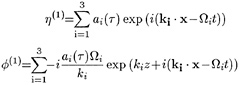 ,
,
where ai are the slowly-varying complex amplitudes of the resonant triad, and ki and Ωi are their respective wavenumbers and wave frequencies, ![]() is a slow time expansion. We could also allow slow variations in space [19] and weak viscous effects [18, 8], but for the purposes of our demonstration a slow-time expansion is sufficient.
is a slow time expansion. We could also allow slow variations in space [19] and weak viscous effects [18, 8], but for the purposes of our demonstration a slow-time expansion is sufficient.
The triad of waves will resonate if the following conditions are satisfied:
k1+k2=k3
Ω1+Ω2=Ω3,
where for deep water, the dispersion relationship is
![]() .
.
At each order of the approximation, evolution equations for ai are derived by eliminating secular terms. These free waves generate bound harmonics. The bound waves are the particular solutions to the governing equations after the secular terms have been eliminated. This solution procedure has been automated using Macsyma, a symbolic algebra code.
We consider a special case that illustrates the directional spreading of wave energy due to triad interactions:
k1=(k1 cos(θ), k1 sin(θ))
k2=(k1 cos(θ), −k1 sin(θ))
k3=(2k1 cos(θ), 0).
where θ is the angle of incidence of the two gravity waves (k1&k2) relative to the capillary wave (k3). The wavenumber that characterizes this case is
Based on the preceding equation, resonance can occur only for cos (θ)<2−1/3 ≈ 37.5deg. These waves are long-crested gravity-capillary waves. The equations that govern the envelop are
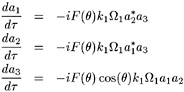 ,
,
where F(θ)=(cos(θ)2+2 cos(θ)−2).
The characteristic velocity is the minimum phase speed for a gravity-capillary wave uc=(4gσ/ρ)1/4. The characteristic length is the inverse wavenumber of this wave ℓc= (σ/ρg)1/2. Based on these scales ![]() and We=2. The solution is inviscid. The angle of incidence is θ=arctan
and We=2. The solution is inviscid. The angle of incidence is θ=arctan![]() . The numerical solution is initialized with ε1=ε2=0.05 and ε3=0. Two hundred time steps are used per gravity-wave period (T=2π/Ω1), and the duration of the simulation is 35 gravity-wave periods. The grid resolution along the x–, y–, & z–axes is 24×48×24. The depth that is used in the numerical simulation is sufficiently deep to neglect finite-depth effects.
. The numerical solution is initialized with ε1=ε2=0.05 and ε3=0. Two hundred time steps are used per gravity-wave period (T=2π/Ω1), and the duration of the simulation is 35 gravity-wave periods. The grid resolution along the x–, y–, & z–axes is 24×48×24. The depth that is used in the numerical simulation is sufficiently deep to neglect finite-depth effects.
Figure 2 compares the modal amplitudes of the analytic and numerical solutions. The agreement is very good initially, but then the solutions begin to diverge after about ten gravity-wave periods. The theory predicts that all of the gravity-wave energy goes into the capillary wave, whereas the numerical solution shows a periodic behavior. This discrepancy is due to a special phase dependence in the analytic theory that can be eliminated by extending the theory to higher order. (We plan to demonstrate this result in a subsequent paper.) The numerical solutions also show a high-frequency behavior due to high-order interactions that are not modeled by the analytic theory. The numerical simulation conserved energy to within four percent after 35 gravity-wave periods (Ɛene(35T)=0.037).
5.4
Test Case IV: Wave-Current Interactions
As a test of the coupling between the potential and vortical portions of our Helmholtz formulation, consider the interaction of a wave with a shear current. A linear analysis of this flow leads to Rayleigh 's stability equation subject to the kinematic and dynamic free-surface boundary conditions [38]. Our current profile has the following general form:
![]() ,
,
where U0 and U1 are the amplitudes of the mean and sinusoidal portions of the current and h is the depth. The characteristic length is the wavelength of the surface disturbance ℓc=λ, and the characteristic velocity is uc= ![]() . The depth is equal to the wavelength. The solution is inviscid and capillarity is not modeled.
. The depth is equal to the wavelength. The solution is inviscid and capillarity is not modeled.
For U1=−U0 the current is highest at the mean free-surface (z=0), and the shear is highest at the mean free surface and the bottom. For our test case all of the eigenvalues are real and the flow is stable. As initial conditions, we choose the eigenmode with the highest eigenvalue. The phase speed of this wave is approximately ![]() . Twenty-four grid points are used per wavelength and one hundred time steps are used per wave period. Two wave steepnesses and two currents are chosen to show the convergence of the fully-nonlinear numerical solution to the linear analytic solution as the steepness and shear are reduced.
. Twenty-four grid points are used per wavelength and one hundred time steps are used per wave period. Two wave steepnesses and two currents are chosen to show the convergence of the fully-nonlinear numerical solution to the linear analytic solution as the steepness and shear are reduced.
Table 4: Wave-current convergence test.
|
U0 |
ε |
εη(T) |
εω(T) |
εene(T) |
|
0.1 |
0.01 |
2.3(−2) |
1.5(−3) |
1.0(−4) |
|
0.1 |
0.02 |
2.5(−2) |
2.9(−3) |
4.5(−4) |
|
0.2 |
0.01 |
4.9(−2) |
2.1(−3) |
7.8(−5) |
|
0.2 |
0.02 |
5.0(−2) |
4.4(−3) |
2.6(−4) |
Table 4 illustrates the convergence of the numerical scheme as a function of the wave
steepness and the shear. The error in the surface vorticity (![]() ω) is normalized by
ω) is normalized by ![]() = |U1|π/2h. The errors in the free-surface elevation are halved when the magnitude of the shear is halved. Similarly, the errors in the surface vorticity are halved when the wave steepness is halved. The kinetic and potential energy is conserved to within .05% for all cases.
= |U1|π/2h. The errors in the free-surface elevation are halved when the magnitude of the shear is halved. Similarly, the errors in the surface vorticity are halved when the wave steepness is halved. The kinetic and potential energy is conserved to within .05% for all cases.
5.5
Test Case V: Gerstner's Wave
Table 5 shows the numerical errors as a function of the spatial and temporal resolution and the nonlinearity when Gerstner's wave is used as initial conditions[12]. A Newton-Raphson technique is used to convert Gerstner's Lagrangian coordinates to our Eulerian coordinates. Then a boundary-value problem is solved to convert from the primitive-variable formulation of Gerstner to our Helmholtz decomposition. The characteristic length is the wavelength ℓc=λ, and the characteristic velocity is ![]() . The depth is equal to the wavelength. The solution is inviscid and rotational. Capillarity is not modeled.
. The depth is equal to the wavelength. The solution is inviscid and rotational. Capillarity is not modeled.
Table 5: Gerstner's wave convergence test.
|
zs |
λ/Δx |
T/Δt |
|
|
|
|
−0.1 |
24 |
50 |
1.9(−2) |
3.0(−2) |
3.1(−2) |
|
−0.1 |
48 |
100 |
7.5(−3) |
7.3(−3) |
1.3(−2) |
|
−0.2 |
24 |
50 |
3.1(−3) |
1.1(−3) |
9.6(−3) |
|
−0.2 |
48 |
100 |
1.2(−3) |
1.7(−4) |
4.3(−3) |
The wave steepness, ![]() , is a function of zs:
, is a function of zs: ![]() , where k is the wavenumber and zs=0 corresponds to a cycloid. The two entries in the table for zs=−0.1 and −0.2 correspond to
, where k is the wavenumber and zs=0 corresponds to a cycloid. The two entries in the table for zs=−0.1 and −0.2 correspond to ![]() =.53 and .28. The error in the surface vorticity is normalized by
=.53 and .28. The error in the surface vorticity is normalized by ![]() , where Ω is the wave frequency.
, where Ω is the wave frequency.
The errors in the surface vorticity show that the fourth-order accuracy is approached as the grid resolution is increased. However, the convergence of the free-surface solution is not as rapid. A closer inspection of the numerical results shows that the cusp that occurs at the crest of the Gerstner wave is smoothed out. Another factor that contributes to the slower convergence is the finite-depth effects that are present in the numerical solution, but not the analytic solution. Even with these limitations, the accuracy of these numerical simulations is comparable to the simpler gravity-wave case.
6
LES PERFORMANCE STUDIES
The LES formulation is tested a priori using a DNS dataset of three-dimensional homogeneous turbulence and a posteriori using numerical simulations of free-surface turbulence. The DNS code that is used to generate the dataset of homogeneous turbulence uses the same finite-difference operators and multigrid solver as the free-surface code. The study of homogeneous turbulence allows us to perform high-resolution simulations of a flow that is less complex than free-surface turbulence. The LES studies of free-surface turbulence include comparisons to moderate-resolution DNS studies of turbulence without waves, turbulence with waves, and waves without turbulence. These numerical simulations allow us to assess the performance of the test-filter approach and the SGS closures under a variety of conditions.
6.1
A Priori Tests
The a priori tests of the SGS models are based on a DNS simulation of homogeneous turbulence. Based on a length scale of ℓc= 5cm and a rms-velocity scale of uc=4cm/s, the Reynolds number is Re=2000. These scales are chosen to match our free-surface turbulence studies, which we will discuss later. As initial conditions, we used white noise with zero mean that was projected onto a solenoidal velocity field. A 1283 numerical simulation was run until the kinetic energy decayed to about 25% of its initial value. Then the velocity field was rescaled so that
the rms velocity was equal to one. This process was repeated until the shape of spectrum did not change. The Taylor Reynolds number at this point was Rλ=46.
Figure 3 compares energy spectrums of numerical simulations to the measurements of Comte-Bellot and Corrsin [2]. The energy density and the wavenumbers are normalized using Kolmogorov units. The numerical simulations include the results of 1283 psuedo-spectral simulations (labeled I and II), and eight-point and six-point upwindbiased finite-difference codes2. The first spectral simulation was allowed to naturally decay. The second spectral simulation forced the lowest wavenumbers to make the spectrum stationary. The six-point FDM scheme is used in our free-surface code. The results of the eight-point FDM scheme are included to illustrate convergence.
The finite-difference codes compare as well to the experiments as the spectral codes. Moreover, the finite-difference codes show no evidence of an energy pileup at the highest wavenumbers, unlike the spectral codes. Except for the energy pileup, a nonstationary spectrum may explain the poorer agreement of the first spectral simulation with the experimental data. The poorer agreement of the second spectral simulation at the lower wavenumbers may be attributed to the forcing. As expected, the eight-point finite-difference scheme shows slightly better agreement with the experimental data at the highest wavenumbers. However, considering that this slight discrepancy is occuring at the Nyquist wavenumbers, the excellent agreement of both finite-difference codes with the experimental data is remarkable. We are currently investigating the performance of the finite-difference codes at higher Reynolds numbers on a CM-5 computer.
The DNS dataset from the eight-point finite-difference code is used to generate synthetic LES velocity fields using different filters. The SGS stress tensor is calculated using the definition in Equation (6). Then volume-averaged SGS coefficients are calculated using Lilly 's least-squares procedure. Table 6 provides the SGS coefficients and the correlation coefficients. The effective lengthscale of each filter is Δe, and Δ is the grid spacing. As the ratio Δe/Δ gets larger, more energy is filtered out. Two of the filters correspond to the grid and test filters that are defined in Equations (22 & 23). The third filter is a very coarse second-order accurate filter. The correlation coefficient is defined below:
![]() , (33)
, (33)
where ![]() is the SGS stress tensor and
is the SGS stress tensor and ![]() is the model SGS stress tensor. The brackets denote volume averaging.
is the model SGS stress tensor. The brackets denote volume averaging.
Table 6: SGS and correlation coefficients.
|
Type |
Δe/Δ |
C1 |
C6 |
C7 |
C(m) |
|
I |
256/193 |
8.10(−3) |
0.06 |
||
|
I |
16/7 |
2.55(−2) |
0.17 |
||
|
I |
16/5 |
5.59(−2) |
0.26 |
||
|
II |
256/193 |
1.20 |
0.95 |
||
|
II |
16/7 |
1.40 |
0.94 |
||
|
II |
16/5 |
1.81 |
0.90 |
||
|
III |
256/193 |
1.92(−4) |
1.20 |
0.95 |
|
|
III |
16/7 |
−5.28(−4) |
1.40 |
0.94 |
|
|
III |
16/5 |
4.72(−3) |
1.80 |
0.90 |
|
|
IV |
256/193 |
−9.81(−3) |
0.25 |
||
|
IV |
16/7 |
−3.94(−2) |
0.69 |
||
|
IV |
16/5 |
−1.36(−1) |
0.87 |
||
|
V |
256/193 |
1.20 |
0.95 |
||
|
V |
16/7 |
1.58 |
0.95 |
||
|
V |
16/5 |
2.20 |
0.98 |
In Table 6 the correlation of the global model (Types II and V) is much better than the local models (Types I and IV), and the combination of a local model with the global model (Type III) does not improve the performance of the global model alone (Type II). In general, the correlations of the global models slightly decrease as the coarseness of the filter increases, whereas the correlations
|
2 |
Dr. Thomas Lund at Nasa Ames provided us with the spectral results. |
of the local models improve. All of the SGS coefficients increase as coarseness increases.
The Type I model with Δe/Δ=16/5 roughly corresponds to one case that Lund and Novikov investigated using a spectral code with a sharp-cutoff filter and volume averaging [13]. For this case their correlation coefficient (C=0.24) agrees with our results. As a possible explanation of the excellent correlation coefficients for the global model, consider the correlation between the energy density (ukuk) and the filtered energy-density ![]() . For even the coarsest filter, this correlation exceeds 0.97. This implies that most of the kinetic energy is concentrated in the lowest wavenumbers, which helps to explain the excellent correlation of the global model. Moreover, as noted by Meneveau, et al (1992), although the global model captures a significant portion of the SGS energy, its wavenumber content is too high to be resolved by a LES formulation [20]. So it is possible for the global model to have a high correlation in a static test, like we have just performed, and still perform less well in a dynamic test as we will see in next section.
. For even the coarsest filter, this correlation exceeds 0.97. This implies that most of the kinetic energy is concentrated in the lowest wavenumbers, which helps to explain the excellent correlation of the global model. Moreover, as noted by Meneveau, et al (1992), although the global model captures a significant portion of the SGS energy, its wavenumber content is too high to be resolved by a LES formulation [20]. So it is possible for the global model to have a high correlation in a static test, like we have just performed, and still perform less well in a dynamic test as we will see in next section.
6.2
A Posteriori Tests
Table 8 in Section 9 at the end of this paper provides the details of six DNS studies of free-surface turbulence. These DNS studies, which include simulations of subsurface turbulence without waves, turbulence with waves, and waves without turbulence, are compared to low-resolution LES. The LES studies and the DNS studies that they are compared to are provided in Table 9.
The initial assignment of the subsurface-velocity field is similar to the procedure Dommermuth (1993a) discusses in his Appendix C [ 6]. The initial shape of the subsurface-velocity spectrum is κ−5/3. The mean velocity components are zero. To ensure that the LES and DNS studies use identical initial conditions, only low wavenumbers (κ≤12π) that will fit into the LES are excited. Free-slip boundary conditions are initially used on the plane z=0. If a surface wave is also present, then the subsurface-velocity field is periodically extended above the plane z=0. A boundary-value problem is solved to set the normal-component of the surface velocity to zero (see Equation 8). The initial rms velocity of the subsurface-velocity field is set to one, whether or not a surface wave is present. The surface wave is assigned using an exact Gravity wave, and the generation of spurious high-frequency waves due to imbalances in the initial conditions is eliminated using an adjustment procedure (see [6], [7], & [8]). The simulations are run for about 2.5 wave periods, or more than two small-scale eddy-turnover times (to) for the lowest Froude-number runs and almost six turnover times for the highest Froude number, where to=λo/uo,λo is the final Taylor microscale, and uo is the final rms velocity.
The spectrum of the total-velocity field is calculated by taking the Fourier transform in the horizontal plane of ![]() where D is the depth and η+D accounts for the vertical extent of the fluid. The Fourier coefficients are squared and integrated over the depth. Finally, the energy density is summed over wavenumber shells to calculate the one-dimensional spectrum E(κ). Details of a similar procedure are provided in Dommermuth (1993a).
where D is the depth and η+D accounts for the vertical extent of the fluid. The Fourier coefficients are squared and integrated over the depth. Finally, the energy density is summed over wavenumber shells to calculate the one-dimensional spectrum E(κ). Details of a similar procedure are provided in Dommermuth (1993a).
Figures 4 & 5 compare the spectra of the DNS to the LES for cases with and without surface waves. Both figures include the spectrum of the total velocity field (E(κ)) and the spectrum of the wave energy (S(κ)). By comparing the initial velocity spectra to the final velocity spectra (see Figures 4a & 5a), we observe that the higher wavenumbers (κ>12π) of the DNS runs have filled in according to Kolmogorov's law (E(κ) ∝ κ−5/3). The spectra of wave energy in Figure 4b show a buildup of energy for wavenumbers κ>2π relative to the initial conditions. This buildup corresponds to the formation of parasitic capillary waves on the front face of the
gravity wave (see [3], [16], & [8]). With no initial wave, the spectra of wave energy correspond to surface roughness (see Section 7.2). Since roughness is proportional to pressure, the spectra of roughness should behave as
![]() ,
,
where the κ−7/3 dependence is associated with the pressure [21] and the denominator includes free-surface effects (see Section 7.2). This trend is illustrated in Figure 5b.
Comparing the LES and DNS velocity spectra in Figures 4a & 5a shows that low-resolution LES (24×24×25) tend to decay less rapidly than the DNS for the lowest few wavenumbers. This anomaly is reduced when the resolution of the LES is increased (see ‘LES 6' run in Figure 5a). We speculate that once a sufficient portion of the turbulent energy cascade is captured by the LES, then this problem will be eliminated. However, we will require DNS with higher resolution or experimental measurements to validate LES with higher resolution.
The higher wavenumbers (κ>12π) of the LES velocity spectra (see Figures 4a & 5a) decay more rapidly than the DNS because the current formulation of the LES applys a grid filter, (see Equation 22). Without the grid filter, the LES break down due to a buildup of energy at the Nyquist wavenumbers. The differences between the SGS models are relatively small. In fact, just the grid filter (LES runs 1, 5, and 6) without a SGS model performs as well as the more complex LES formulations (LES runs 2–4). Whether this trend will continue at higher resolution is not clear.
The dissipation in a LES is provided by the SGS model, the viscous terms in the Navier-Stokes equations, and the grid filter. The grid filter for the low-resolution LES provides about 75% of the dissipation, 20% is provided by the viscous terms, and the final 5% is provided by the SGS models. However, the global SGS model (Type II) sometimes provides a small net increase in energy (see LES run 2). The inclusion of the Smagorinsky model (Type III) does not reverse this trend in a test filter approach because the global model dominates (see LES run 3). This dominant behavior is also observed in the a priori tests. The Smagorinsky model (Type I) always provided some dissipation. This explains why the low wavenumbers associated with this model agree slightly better with the DNS (see LES run 4 in Figure 4a).
The volume-averaged coefficient of the global model is nearly constant (c7≈1.0) during the simulations (LES runs 2 & 3) for both the anisotropic and isotropic portions of the SGS stresses. The Smagorinsky coefficient rises to a peak value of about c1=0.36 during the developing stage of the flow (LES run 4), and then steadily decreases to a value of c1=0.22 at the end of the simulation. When the Smagorinsky model is used in combination with the global model (LES run 3), the magnitude of the Smagorinsky coefficient is an order of magnitude less and its sign varies. The coefficient of the isotropic model (Type IV) is almost constant (c6=−0.60, LES run 4). Overall, the coefficient's magnitudes are higher than what we had expected based on the a priori tests. As the resolution of the LES increases, we conjecture that the magnitude of the coefficients will go down.
Figures 6a-d compare LES and DNS free-surface cuts as a packet of parasitic capillary waves forms on the front face of the gravity wave. The wave is propagating from right to left. The initial conditions are a pure gravity wave (see parts a & b), and the parasitic capillary waves form from rest due to a parametric resonance near the crest (see parts c & d). The wave length of the ripples is determined by the condition that the phase velocity of the ripples is equal to the phase velocity of the gravity wave plus the local water-particle velocity of the gravity wave [16]. When the subsurface flow is free of turbulence, the 5cm
wave that is modeled in Figures 6a-d will form nine ripples on the front face of the gravity wave, and the wavelength and the amplitude of these ripples will steadily decrease down the face of the gravity wave [8].
Although LES cannot resolve the ripples that are observed in the DNS data that is plotted in Figures 6c & d, Part (d) shows that the ‘mean' slope is predicted well by the LES. Since the attenuation of wave energy due to viscosity is proportional to the wavenumber squared, the inability of the LES to resolve the ripples could give the wrong wave dissipation. This effect may explain why the LES predicts a slightly higher wave amplitude than the DNS (see Figure 6c). This mechanism for wave dissipation is a very sensitive function of the gravity wave's steepness, and it warrants additional investigation using LES with higher resolution.
For these low-resolution LES the wavy portion of the flow is not separated from the vortical flow in the SGS stress models. As our modeling capabilities improve, this separation may be required to model the different physical processes that are associated with the different components of the flow. Our Helmholtz formulation provides a natural technique for performing this separation.
7
NUMERICAL RESULTS
Based on a combination of model-scale measurements and numerical predictions of the Taylor length scale and the rms turbulent velocity in a ship wake, we expect Taylor Reynolds numbers Rλ=O(105−106) and Taylor Froude numbers Fλ=O(10−1−10−3) that depend on the distance aft. We do not expect strong interactions between the subsurface turbulence and the surface waves in the far wake of the ship, where the Froude number is low, but we still need to quantify the types of interactions and their behavior as a function of the Froude number. Here, we use the results of the DNS to investigate the structure of turbulence near the free surface, turbulent roughening of the free surface, and turbulent scattering and dissipation of waves at the low Taylor Froude numbers (O(10−1−10−2)) that would occur several ship lengths astern of the ship. The longest wave lengths that we model correspond to a C-Band radar at an angle of incidence of 30 degrees. The numerical details of the DNS are provided in Table 8 in Section 9 at the end of this paper.
As the characteristic velocity and length scales, we choose the rms velocity of the turbulence and the wavelength of the ambient wave. In physical units, we simulate rms turbulence velocities from 2– 4cm/s interacting with a 5cm gravity-capillary wave. This leads to Taylor Reynolds of Rλ=O(50–100). Based on our earlier simulations of homogeneous turbulence (see §6.1, the resolution of the bulk flow is adequate. The free-surface boundary layer, however, is not resolved. Since our primary goal is to model the work that the turbulence performs on the waves, we choose to use the DNS free-surface boundary conditions (see Equation 10) as if the boundary-layer is fully resolved. (For example, the prediction of turbulent roughening of the free surface does not require resolving the free-surface boundary layer, see Section 7.2.) Upon further validation of our free-surface boundary-layer formulation (see Equation 11), we will incorporate that capability into our DNS code. A preliminary validation study is provided in Dommermuth (1993c).
7.1
The Turbulent Structure Near the Free Surface
Laboratory measurements of a turbulent vortex-tube interacting with a free surface show the formation of whirls [32, 33]. The observed persistence and amalgamation of these whirls is characteristic of two-dimensional turbulence. Whether this behavior is common to turbulent free-surface flows in general is questionable because this particular
vortex-tube experiment had a moving stagnation point on the free surface where the whirls would naturally tend to collect [31, 5, 6]. This issue is addressed using a DNS of a more general turbulent free-surface flow.
For any function F(x,y,z,t) such as vorticity, we can define an one-dimensional energy operator (E1d):
![]() ,
,
where ![]() is a mapping, and D is the depth. (The free surface corresponds to
is a mapping, and D is the depth. (The free surface corresponds to ![]() and z=η, and the bottom corresponds to
and z=η, and the bottom corresponds to ![]() and z=−D.) The operator E1d provides a vertical distribution of energy for a function F. An integral of E1d with respect to
and z=−D.) The operator E1d provides a vertical distribution of energy for a function F. An integral of E1d with respect to ![]() multiplied by the depth D provides the total energy in the fluid volume.
multiplied by the depth D provides the total energy in the fluid volume.
Figures 7a & b provide the enstrophy distribution for the vertical component of vorticity (E1d(ωz)) and the energy distribution for the horizontal components of velocity (E1d(u)+E1d(ν)). The vertical component of vorticity corresponds to the whirls that are observed in laboratory experiments. As time increases, Figure 7a shows that E1d(ωz), after a small initial increase, actually decreases by about 25% near the free surface (![]() ) and the free-slip bottom (
) and the free-slip bottom (![]() ). In the interior of the fluid for
). In the interior of the fluid for ![]() =0.75, 0.50, and 0.25 the enstrophy increases and actually more than doubles in one case. There is no evidence that the vertical component of vorticity tends to persist longer at the free surface for this low Reynolds number simulation.
=0.75, 0.50, and 0.25 the enstrophy increases and actually more than doubles in one case. There is no evidence that the vertical component of vorticity tends to persist longer at the free surface for this low Reynolds number simulation.
Figure 7b shows that the horizontal velocity components have at least 50% more energy near the free surface and the free-slip bottom than in the interior of the flow. The high velocities near the boundaries of the fluid are due to horizontal vortices interacting with their images. These high horizontal velocities may actually inhibit the connection of normal vorticity with the free surface. Granted, these results are for a single realization of a turbulent flow at a low Reynolds number, but they do not support the notion that the flow near the free surface behaves like two-dimensional turbulence.
7.2
Free-Surface Roughness
We define roughness as the free-surface disturbance that is caused by subsurface turbulence in the absence of ambient waves. At low Froude numbers, the free-surface elevation is hydrostatically balanced with the component of the pressure that is induced by the vortical portion of the flow:
![]() . (34)
. (34)
If capillarity is important, then
![]() , (35)
, (35)
where the hat symbol (^) denotes the Fourier transform and κ is the horizontal wavenumber. As the Froude number increases, dispersive effects may become important, then
(36)
where ![]() is the wave frequency.
is the wave frequency.
In Table 7 we compare the preceding formulas to two DNS of a fully-nonlinear free-surface flow (see Runs 1 & 4 in Table 8). Two additional DNS with free-slip boundary conditions on the “free surface” are used to calculate the vortical component of the pressure. This pressure is inserted into the three formulas for roughness. Table 7 provides the correlation coefficients between the free-surface and free-slip wall calculations. The symbols C34, C35, and C36 respectively correspond to the correlation coefficients for Equations (34, 35, & 36). The results are for the final time step.
Table 7: Roughness correlation coefficients.
|
DNS Run |
C34 |
C35 |
C36 |
|
1 |
0.939 |
0.998 |
0.999 |
|
4 |
0.767 |
0.907 |
0.928 |
The correlation coefficients for DNS Run 1 are better than DNS Run 4 because Run 1 has a lower Froude number and less nonlinearity. Comparing the coeffients C35 to C34 in Table 7 shows that capillary effects are important for the 5cm and smaller disturbances that Runs 1 and 4 model. Dispersive effects do not appear to be as important because the C36 coefficients are only slightly better than the C35 coefficients. Overall, the good agreement of the free-slip-wall simulations with the fully-nonlinear free-surface simulations provides strong support for using simple free-slip-wall formulations to perform roughness calculations.
7.3
Turbulent Scattering of Waves
We define turbulent scattering as the directional spreading of surface waves due to interactions with subsurface turbulence. In our simulations the surface wave is initially propagating along the x—axis, and then the interactions of the wave with the turbulence move wave energy off of the x—axis. One measure of how much scattering has occurred in our numerical simulations is the amount of potential energy that has nonzero y—wavenumbers, which we denote as Es. The operator Es also includes the effects of roughness, but its effect on Es is minimal because the total potential energy due to roughness is less than 0.2% of the wave potential energy.
Figure 8 plots the turbulent scattering of wave energy for the two different Froude numbers in Table 8. The two curves are initially flat due to the effects of the adjustment procedure, but then the slopes of the curves develop a mean component. The slope of the fitted curve in the figure is equal to the mean slope of the numerical data. Based on this fitted curve, we estimate that the rate of turbulent scattering (μs) is
![]() , (37)
, (37)
where Ep is the initial potential energy. (Note that the time t is normalized by the ratio of the rms turbulent velocity to the wavelength.) Equation (37) represents a spreading of wave energy that can act like an apparent dissipation. Let Eo equal the total wave energy, which includes the kinetic, potential, and superficial energy, then the laminar rate of energy decay (μl) is
![]() , (38)
, (38)
where κ=2π is the wavenumber of the surface wave. If we assume that the scattering formula in Equation (37) is equally valid for the kinetic and superficial energy components, then for a Reynolds number Re= O(103), the apparent dissipation due to scattering is the same order as the attenuation due to laminar decay.
Another scattering mechanism that is important for gravity-capillary waves is the triad resonance that is discussed in Section 5.3. The rate of scattering of wave energy due to a triad resonance (μr) is proportional to the wave steepness (μr α κa, where κ is the wavenumber and a is the wave amplitude). For short steep waves, especially wind-driven waves, this mechanism is as effective as turbulence for scattering wave energy. This is illustrated in Figure 2, where we observe that over 75% of the gravity-wave energy has scattered after only fifteen wave periods. However, triad resonances, unlike turbulent scattering, have a nonlinear recurrence that may limit their overall effectiveness.
Figure 9 plots the x-component of the free-surface slope for two different Froude numbers at roughly the same nondimensional time t/Fr=8.35. The scattered potential energies relative to the initial potential wave energies are the same order at this time. This
indicates that the long, energy-containing waves, are about equally scattered. We observe, however, that the short parasitic capillary waves are steeper and appear to be more scattered for the higher Froude number case. This is confirmed by analysis of two-dimensional wave spectra. The waves are propagating from right to left along the x—axis.
7.4
Turbulent Dissipation of Waves
We define turbulent dissipation as the attenuation of surface waves due to interactions with subsurface turbulence. The total wave energy Ew is
where the first three terms on the right-hand side of the equation are respectively the wave kinetic energy, the wave potential energy, and the wave superficial energy. Let Ew1, Ew2, and Ew3 respectively represent the energy with an ambient wave but no turbulence, the energy with an ambient wave and turbulence, and the energy with turbulence but no ambient wave. We define the change of wave energy (Ed) due to the actions of turbulence as
Ed=Ew1−(Ew2−Ew3).
In our DNS runs, we neglect Ew3 because it never exceeds .2% of Eo, where Eo is the initial value of Ew1.
Figure 10 plots the turbulent dissipation of the wave energy for the two different Froude numbers in Table 8. The two curves are initially flat due to the effects of the adjustment procedure, but then the slopes of the curves develop an oscillatory and a mean component.
The period of the oscillations is roughly equal to the wave period, which would suggest that the amplitude of the oscillations is proportional to the wave amplitude. This possible dependency will be investigated in a future paper.
The mean offset in the slope represents a net decrease in the wave energy. The slope of the fitted curve in the figure is equal to the mean slope of the numerical data. Based on this fitted curve, we estimate that the turbulent dissipation rate (μt) is
μt=4EoFr. (39)
Comparing the turbulent dissipation rate relative to the turbulent scattering rate shows that turbulent dissipation decreases more rapidly as the Froude number decreases (see Equation 37). For Froude numbers O(10−1− 10−2), the turbulent dissipation rate is the same order as the turbulent scattering rate and the laminar dissipation rate (see Equation 38). However, all of these effects are less than the dissipation rates associated with the formation of parasitic capillary waves (μc) and the effects of surfactant films (μf).
In the case of parasitic capillary waves, Dommermuth's numerical simulations and Longuet Higgins' theoretical predictions show that μc=O(5μl−10μl) for steep 5cm gravity capillary waves [8, 16]. Pillips shows that in the inextensible limit of a surfactant film that μf=O(10μl) for a 5cm gravity-capillary wave [29].
Our turbulent-dissipation rate is four times lower than the dissipation rate that Olmez & Milgram (1992) measure [28]. We note, however, that the laminar decay rate that they measure is two times higher than theory. Two possible explanations that could explain the differences between our predictions, their measurements, and theory include the effects of the poor resolution of the free-surface boundary layer in the numerical simulations and the effects of a surfactant film that may have been present in the Michi-
gan towing-tank facility even with the use of scrubbers3.
8
CONCLUSIONS
Comparisons between the LES and DNS indicate that the LES should be performed at higher resolution to resolve a sufficient portion of the turbulent energy cascade. For the present low-resolution LES, the global stress model (Type II closure) provides excellent prediction of the SGS stresses, but the wavenumber content is too high to be resolved in a LES formulation. For the same resolution, a grid filter with no SGS model works as well as the closure models that we have tested to date. These trends require investigation at higher resolution. The next step in SGS modeling will also require a detailed study of the structure of turbulence [25, 27].
DNS studies of free-surface turbulence do not provide evidence that whirls will persist on the free surface due to the effects of two-dimensional turbulence at low Reynolds numbers. DNS studies show that free-surface roughness is proportional to the component of the pressure that is induced by the vortical portion of the flow. Since turbulent dissipation relative to turbulent scattering is a higher order function of the Froude number, its effects will diminish more rapidly in a ship wake. The turbulent scattering and dissipation of 5cm surface waves are dominated by the effects of parasitic capillary waves and surfactants for Froude numbers that would correspond to a region that is several ship lengths aft of the stern.
These DNS results are tempered by our inability to resolve the free-surface boundary layer. We propose to overcome this problem by using the boundary-layer formulation of the free-surface boundary conditions that we provide in Equation (11). This boundary condition is already incorporated into our LES capability. The boundary-layer formulation enables us to simulate the dominate dissipative effects of parasitic capillary waves while still maintaining an ability to predict free-surface roughness, and turbulent scattering and dissipation.
ACKNOWLEDGEMENTS
This research is financially supported by the Fluid Dynamics Program at the Office of Naval Research. E.A.N. is also supported by the Department of Energy. The numerical simulations have been performed on the CRAY Y-MP's at the Numerical Aerodynamic Simulation (NAS) Program and the Primary Oceanographic Prediction System (POPS), and the CM-5 at the Naval Research Laboratory. We are grateful to Dr. Thomas Lund at Nasa Ames Research Center, who provided us with the results of spectral computations. We are also indebted to Dr. Robert Hall at Science Applications International Corporation for his helpful discussions.
References
[1] Bardina, J., Ferziger, J.H., and Reynolds, W.C. ( 1980) Improved subgrid-scale models for large-eddy simulations. AIAA 80–1357.
[2] Comte-Bellot, G. and Corrsin, S. ( 1971) Simple Eulerian time correlation of full and narrow-band velocity signals in grid-generated ‘isotropic' turbulence. J. Fluid Mech., 48, 273–337.
[3] Cox, C.S. ( 1958) Measurements of slopes of high-frequency wind waves. J. Mar. Res, 16, 199–225.
[4] Deardorff, J.W. ( 1970) A numerical study of three-dimensional turbulent channel-flow at large Reynolds numbers. J. Fluid Mech., 41, 453–480.
[5] Dommermuth, D.G. ( 1992) The formation of U-shaped vortices on vortex tubes impinging on a wall with applications to free surfaces. Phys. Fluids, A bf 4(4), 757–769.
[6] Dommermuth, D.G. ( 1993a) The laminar interactions of a pair of vortex tubes with a free surface . J. Fluid Mech., 246, 91–115.
[7] Dommermuth, D.G. ( 1993b) The initialization of vortical free-surface flows. J. Fluids Eng. To appear.
|
3 |
In a private conversation, Prof. Milgram noted that he has since measured dissipation rates in another facility that are similar to his previous measurements. |
[8] Dommermuth, D.G. ( 1993c) Efficient Simulation of short- and long-wave interactions with applications to capillary waves. J. Fluids Eng. To appear.
[9] Germano, M., Piomelli, U., Moin, P., and Cabot, W.H. ( 1991) A dynamic subgrid-scale eddy viscosity model. Phys. Fluids, A 3(7), 1760–1765.
[10] Gharib, M., Wegand, A., Dabiri, D., and Novikov, E. ( 1993) Interaction of small-scale turbulence with a free surface. Submitted for publication.
[11] Hirt, C.W., Nichols, B.D., and Romero, N.C. ( 1975) SOLA-A numerical solution algorithm for transient fluid flows. Los Alamos Scientific Lab. Report No. LA-5852.
[12] Lamb, H. ( 1932) Hydrodynamics. Dover.
[13] Lund, T.S. and Novikov, E.A. ( 1992) Parameterization of subgrid-scale stress by the velocity gradient tensor. In Annual Research Briefs. Center for Turbulence Research, NASA-Ames Research Center and Stanford University.
[14] Leighton, R.I., Swean, T.F., Handler, R.A., and Swearingen, J.D. ( 1991) Interaction of vorticity with a free surface in turbulent open channel flow. In Proceedings of the 29th Aerospace Sciences Meeting, Reno, NV, AIAA 91–0236.
[15] Lilly, D.K. ( 1991) A proposed modification of the Germano subgrid-scale closure method . Phys. Fluids, A 4(3), 633–635.
[16] Longuet-Higgins, M.S. ( 1963) The generation of capillary waves by steep gravity waves. J. Fluid Mech., 16, 138–159.
[17] Longuet-Higgins, M.S. ( 1991) Theory of weakly damped Stokes waves: a new formulation and its physical interpretation. J. Fluid Mech., preprint.
[18] Lundgren, T.S. ( 1989) A free-surface vortex method with weak viscous effects. In Mathematical Aspects of Vortex Dynamics, ed. by R.E.Caflisch, SIAM, pp. 68–79.
[19] McGoldrick, L.F. ( 1970) On Wilton's ripples: a special case of resonant interactions. J. Fluid Mech. 42, 193–200.
[20] Meneveau, C., Lund, T.S., and Moin, P. ( 1992) Search for subgrid scale parameterization by projection pursuit regression . In Studying Turbulence Using Numerical Simulation Databases -IV. Center for Turbulence Research, NASA-Ames Research Center and Stanford University.
[21] Monin, A.S. and Yaglom, A.M. ( 1975) Statistical Fluid Mechanics II. The MIT Press, Cambridge, MA
[22] Moin, P. ( 1990) I. The subgrid scale modeling group. In Studying Turbulence Using Numerical Simulation Databases—III, Proceedings of the 1990 Summer Program. Center for Turbulence Research, NASA-Ames Research Center and Stanford University.
[23] Novikov, E.A. ( 1991) Solutions of exact kinetic equations for intermittent turbulence. In Monte-Verita Symposium on Turbulence, Switzerland, preprint.
[24] Novikov, E.A. ( 1992a) Self-amplification of turbulent 3D vorticity field and 2D vorticity gradient. J. Phys., A 25, 657.
[25] Novikov, E.A. ( 1992b) Probability distributions for three-dimensional vectors of velocity increments in turbulent flow. Phys. Rev. A, Rapid Comm., 46 (10), R6147.
[26] Novikov, E.A. ( 1993a) A new approach to the problem of turbulence, based on the conditionally-averaged Navier-Stokes equations. Fluid Dyn. Res., 12 (10).
[27] Novikov, E.A. ( 1993b) Statistical balance of vorticity and a new scale for vortical structures in turbulence. Phys. Rev. Let., Submitted.
[28] Olmez, H.S. and Milgram, J.H. ( 1992) An experimental study of attenuation of short water waves by turbulence . J. Fluid Mech., 239, 133–156.
[29] Phillips, O.M. ( 1980) The Dynamics of the Upper Ocean. Cambridge University Press.
[30] Rai, M.M and Moin, P. ( 1991) Direct simulations of turbulent flow using finite-difference schemes . J. Comp. Phys., 96, 15–53.
[31] Sarpkaya, T. and Suthon, P. ( 1991) Interaction of a vortex couple with a free surface. Exp. Fluids, 11 205–217.
[32] Sarpkaya, T. ( 1992) Interaction of a turbulent vortex with a free surface. In Proc. 19th Symp. on Naval Hydro., Seoul, Korea.
[33] Sarpkaya, T. ( 1992) Three-dimensional interactions of vortices with a free surface. In Proceedings of the 30th Aerospace Sciences Meeting, Reno, NV, AIAA 92–0059.
[34] Schumann, U. ( 1975) Subgrid scale model for finite difference simulations of turbulent flows in plane channels and annuli. J. Comp. Phys., 18, 376– 404.
[35] Schwartz, L.W. ( 1974) Computer extension and analytic continuation of Stokes' expansion for gravity waves. J. Fluid Mech., 62, 553–578.
[36] Smagorinsky, J. ( 1963) General circulation experiments with the primitive equations. Mon. Weather Rev., 91, 99–164.
[37] Speziale, C.G. ( 1985) Galilean invariance of subgrid-scale stress models. J. Fluid Mech., 156, 55.
[38] Triantafyllou, G.S. and Dimas, A.A. ( 1989) Interaction of two-dimensional separated flows with a free surface at low Froude numbers. Phys. Fluids, A 1(11), 1813–1821.
[39] Zhang, Y., Street, R.L., and Koseff, J.R. ( 1993) Thoughts on the development of a dynamic subgrid-scale model for free- surface flow. In 1993 Free-Surface Vorticity Workshop, Pasadena.
9
TABLES
Table 8: Data for DNS runs.
The ‘Includes Wave?' item indicates whether a fully-nonlinear gravity wave is present in the initial conditions. Similarly, the ‘Includes Turbulence?' item indicates whether the initial conditions include a subsurface-velocity field. The length of the wave is ℓc and the initial rms velocity of the subsurface velocity field is uc. H/λ=H/ℓc is the initial wave steepness. Re, Fr, and We are respectively the Reynolds, Froude, and Weber numbers based on the characteristic scales ℓc and uc. Rλ is the Taylor Reynolds number at the final time step. The time step is Δt, and Nt is the number of time steps. The adjustment factor is δt (see [6]). The component of the pressure that is induced by the vortical flow, the viscous normal stresses, and the effects of capillarity are all adjusted4. The length (x), width (y), and depth (z) of the computation domain are respectively L=1, W=1, and D=1. The number of grid points along the x-,y-, and z-axes are respectively Imax=96 , Jmax=96 , and Kmax=97. The maximum allowable wavenumber in the free-surface elevation is κmax = 64π. Wavenumbers that exceed this value are bandpassed filtered. Three multigrid iterations and six V-cycle Jacobi iterations are used to solve the elliptic equations (see [8]).
Table 9: Data for LES runs.
|
LES 1 |
LES 2 |
LES 3 |
LES 4 |
LES 5 |
LES 6 |
|
|
DNS Run |
6 |
6 |
6 |
6 |
4 |
6 |
|
Model Types |
VI |
II & V |
III & V |
I & IV |
VI |
VI |
|
Resolution |
24×24×25 |
24×24×25 |
24×24×25 |
24×24×25 |
24×24×25 |
48×48×49 |
|
κmax |
24π |
24π |
24π |
24π |
24π |
32π |
|
Δt |
0.0012 |
0.0012 |
0.0012 |
0.0012 |
0.0012 |
0.0009 |
The ‘DNS Run' item is the DNS run in Table 8 that corresponds to the LES run. The ‘Model Types' item is the SGS Model from Table 1 that is used in the LES. The resolution is the number of grid points along the x-, y-, and z-axes. The maximum allowable wavenumber in the free-surface elevation is κmax. Wavenumbers that exceed this value are bandpassed filtered. Δt is the time step. All of the LES runs use 601 time steps.
|
4 |
The adjustment procedure uses an exponential function |


Figure 5: Comparison of DNS and LES Spectra. Initial conditions include subsurface turbulence without a surface wave. (a) Total-velocity spectra at time t= 0.36. (b) Wave energy spectra at time t=0.36. The initial conditions for the total-velocity spectrum are shown. The initial wave energy is zero, corresponding to no wave.


DISCUSSION
by Dr. Thomas T.Huang, David Taylor Model basin
Did you define or quantify the characteristics of numerical dissipation in comparison with the physical dissipation you presented in the paper?
Author's Reply
The numerical validation studies that we performed indicate that numerical dissipation is minimal.
DISCUSSION
by Dr. H.Haussling, Naval Surface Warfare Center
The authors have presented impressive results which help us understand the interactions of turbulence with a free surface. When the decomposition of the pressure field was described in the talk, it was mentioned that this decomposition might be useful in Reynolds-averaged Navier-Stokes computations about ships. Could this suggestion be discussed in more detail?
Author's Reply
A Helmholtz decomposition provides a rigorous treatment of the intersection of the ship hull with the free surface. As a result, unlike conventional RANS techniques, extrapolation is not required to project velocities from the free surface onto the ship hull where the no-slip condition is satisfied. This extrapolation is required in RANS simulations because otherwise the free-surface could not rise up the hull.
The Helmholtz formulation decomposes the flow field into its wavy and vortical parts. The wavy portion (f) of the flow allows the free surface to rise up the wall, and the vortical portion (![]() ) of the flow enforces the no-slip condition on the wall. Since the flow is decomposed into two parts, an additional kinematic boundary condition is required on the free surface. For small free-surface slopes, this additional boundary condition is approximately that the vertical component of the vortical flow is (W≈O). The noslip condition on the wall requires that
) of the flow enforces the no-slip condition on the wall. Since the flow is decomposed into two parts, an additional kinematic boundary condition is required on the free surface. For small free-surface slopes, this additional boundary condition is approximately that the vertical component of the vortical flow is (W≈O). The noslip condition on the wall requires that ![]() .
.
A Helmholtz formulation also allows the use of boundary -layer approximations in the free-surface boundary conditions. This prevents the excessive dissipation of waves that is observed in RANS simulations of free-surface flows.
Computation of Free-Surface Flows Around 3-D Hydrofoil and Wigley Ship by N-S Solver
S.H.Kwag and K.S.Min
(Hyundai Maritime Research Institute, Korea)
ABSTRACT
Computations are carried out to simulate the free-surface flows around the Wigley model. The Navier-Stokes equation is solved by a SIAF (semi-implicit approximate factorization) method where the body-fitted coordinate system and the wall function are invoked. The numerical merit is that each line of block pentadiagonal system is decoupled from others and highly vectorized coding is possible. Calculations are made at the Reynolds number of 106 and the Froude numbers are 0.25, 0.289 and 0.316. The free-surface waves are compared with those by the explicit method and experiments. In the latter part, the flow characteristics of 3-D submerged foil is investigated Flows of five different cases are simulated and compared each other to discuss the free-surface effect on the hydrofoils where the submergence depth and angle of attack are imposed. Through the numerical simulation, it is found that the lift and drag are seriously influenced by the free-surface waves. The righting moment, which comes from the non-symmetrical lift distribution along the span, is also calculated for the heeled case.
NOMENCLATURE
|
Φ |
: non-dimensional pressure |
|
Re |
: Reynolds number, Uo·L/ν |
|
Fn |
: Froude number, |
|
Δt |
: time increment |
|
U,V,W |
: contravariant velocities |
|
q |
: velocity vector in matrix form |
|
ζ |
: free-surface amplitude |
|
K |
: pressure gradient term |
|
n |
: nth time step |
|
L |
: ship length or chord length |
INTRODUCTION
Free-surface flow around ship is one of the most complicated flows because there are various nonlinear phenomena and viscous -inviscid interaction. Recently, with the aid of the rapid development of computer technology, methods called NS solvers, in which the governing equations of the flow are discretized and computed, have become very popular 1–5. Among them, the finite-difference solution methods for the Navier-Stokes equation with free-surface seem to be the most promising because of their generality. However, there are much more difficulties to be overcome in the development of free-surface flow solvers such as the treatment of free-surface boundary condition, especially the viscous and turbulence conditions on the free-surface. Another shortcoming is a long computation time.
In the present paper, the explicit finite-difference method for the Navier-Stokes solver6, is extended to the semi-implicit approximation method The advantage of the present method7 is that the partial differential equations are changed to the ordinary ones. The equations form a system with block pentadiagonal matrices in three dimensional case and can be efficiently solved. Through the
approximate factorization, each line of block system in any of the three sweeps is completely decoupled from others and therefore highly vectorized coding is possible. Through the numerical study, it is confirmed that the present method is very efficient in reducing the computation time and also keeping the accuracy in the results. The computation time can be reduced to a large extent because the marching time interval is increased to several times in the magnitude. It is because the method is, by nature, unconditionally stable. This numerical merit encourages us to challenge the full-scale computation with free-surface.
In the latter part, the free-surface interaction is investigated for 3-D submerged hydrofoil because there is a recent trend to develop high speed ships such as the hydrofoil craft. Duncan8 and Coleman9 made some experiments on the 2-D wings and discussed the flow characteristics as well as the wave breaking. The pressure data are available from Nishiyama10. The calculation results can be seen in Suzuki et al11 through the FDM and BEM analyses even though they are 2-dimensional. Hino12 and Mori13 solved 2-dimensional N-S and Euler equations with the nonlinear free-surface conditions and reviewed on the submerged advancing hydrofoil by calculating the lift and drag forces. In the ship hydrodynamics, the wing is strongly affected by the free-surface and vice versa because the wing usually works near the free-surface. In spite of many research works, there are still a lot of unclear problems. In this sense, it is no doubt necessary to investigate the interaction between the lifting body and free-surface. One of the motivations for the present 3-D lifting body research is that, if we directly solve the N-S equation, there is no need to introduce the so-called Kutta condition which is obscure in 3-D cases. Many researchers have tried to solve the problems by the potential flow approach in which an appropriate modelling of the wake leaving from the trailing edge of the wing is necessary or the wake is solved iteratively. A difficulty is to find a universal and exact model for the Kutta condition. The N-S solver does not include such a problem if the no-slip condition is imposed on the body surface. The no-slip condition used for the viscous flow simulation realizes the shock-free condition for the pressure. The 3-D effect is simultaneously investigated besides the study of interaction with free-surface. The tip vortex, which is a part of the results, shows that the rotational magnitude of velocity is much affected by the submergence depth and 3-dimensionality of the wing. As concerns the resistance, the induced drag is intrinsically explained because it may be an inherent component of forming the pressure drag. The nonlinear property of waves and the interaction of a viscous flow with waves render the fluid motion much more difficult to simulate numerically.
NUMERICAL SIMULATION OF SHIP WAVES
Basic Equation
Numerical simulation of 3-D free-surface flow is carried out by solving the N-S equation basically following to the MAC method. The mean velocity components u, v and w exclusive of the fluctuation components at (n+1) time step are determined by using a forward-time difference as follows.
(1)
where
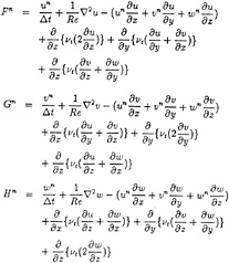
(2)
and
(3)
All the variables are on the cartesian coordinate system(x, y, z) where x is in the uniform flow direction, y in the lateral, and z in the vertical direction respectively ; u, v and w are the velocity components in the x–, y– and z– direction, respectively. They are normalized by the representative length and reference velocity. Subscripts denote the differentiations with respect to the referred variables and superscripts the values at the referred time step. The term Δt stands for the time increment, p the pressure and νt the eddy viscosity. Re and Fn are Reynolds and Froude numbers respectively based on L and Uo, and
(4)
Differentiating (1) with respect to x, y and z, we can have
(5)
The last term in (5) is expected to satisfy the continuity condition. (5) can be solved by the relaxation method The new free-surface at the (n+1)th time-step is calculated by moving the marker particles by
xn+1=xn+unΔt
yn+1=yn+νnΔt
zn+1=zn+wnΔt
(6)
The oncoming flow is accelerated from zero to the given constant velocity. Third-order upstream differencing is used for the convection terms with the fourth-order truncation error which is written as, for example;
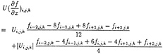
(7)
SIAF Scheme
To solve the N-S equations more efficiently, the SIAF method is used The 3-D equations are used in the computation, but 2-D basic equations are only described for brief understanding. The turbulence model is not particularly remarked here because of the same applicability as in the explicit method. The N-S equation can be written in the non-conservative vector form as follows.
(8)
where
(9)
The numerically-generated, body-fitted coordinate system gives the transformation.
ξ=ξ(x,z,t)
ζ=ζ(x,z,t)
t=t
(10)
It offers the advantages of generality and flexibility and, most importantly, transforms the computational domain into a simple rectangular region with equal grid spacing. Through transformations, (8) can be written for the velocity component q as
(11)
where U and W are the unsealed contravariant velocity components and K′ is transformed from K in terms of (ξ,ζ)

(12)
The Laplacian operator gives


(13)
The implicit form of (11) is as follows.
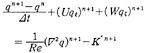
(14)
The (n) and (n+1) mean the time-step, where the value at (n+1) is treated as unknown. The linearization and truncation give

(15)
The convective terms can be written as

(16)
The finite-difference scheme gives
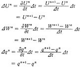
(17)
The governing equation is written as
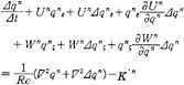
(18)
In above equation, K′(n+1) is approximated as K′(n) because it is not easy to get the solution at the (n+1) time step. The fourth and seventh terms of above equation are approximately factored.
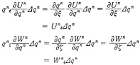
(19)
Rearranging (18) with respect to Δqn, we get
(20)
Here it is not possible to calculate Δqn in the above equation. It is approximated as

(21)
Therefore, through the approximate factorization, the partial differential equations are changed to the ordinary ones.
(22)
The above set of equations form a system with block pentadiagonal matrices in three dimensional case and can be efficiently solved. Through an approximate factorization, each line
of block pentadiagonal system in any of the three sweeps is decoupled completely from others, and therefore highly vectorized coding is possible.
Boundary Conditions
-
On the free-surface, the boundary condition requires zero tangential stress and a normal stress which balances any externally applied forces. The application of these conditions requires a knowledge of not only the location of the free-surface at each grid but also its slope and curvature. In the present calculation, the shape of the free-surface is not known a priori; it is defined by the position of the marker particles. The z-coordinate of the free-surface is rearranged by a linear interpolation in proportion to the newly calculated projected area at each time step. On the free-surface, the exact pressure condition is imposed because the uppermost grid is always identical to the free-surface. By this scheme, it is expected that the free-surface condition, i.e., the constant pressure condition, can be directly applied.
-
On the body surface, the wall function approach is used to reduce the computation time. With the wall condition, the minimum grid spacing in the direction normal to the body surface should be small enough to resolve the viscous sublayer in the boundary layer.
-
At upstream boundary, the uniform flow condition is used; Δq=0. At downstream boundary, zero extrapolation in ξ-direction is used. On the symmetric plane, qη=0 and Δqη =0 is applied At outer boundary, the zero-gradient extrapolation is used.
Turbulence Model
The turbulence model used is the Baldwin-Lomax zero-equation algebraic model, whose original form is the Cebeci-Smith model. It is widely used in the aerodynamic computation and also in the incompressible flow computation around a ship. In the present study, flow is enforced to be turbulent from the fore end of a ship. The free-surface effect on turbulence is not included in the model. There has not been any turbulence model that can be well applied to the boundary layer and wake of a surface-piercing body like a ship. Therefore, in the present calculation, the simple zero equation model is used
COMPUTED RESULTS
Wigley Case
The SIAF method is applied to Wigley model with free-surface. The aim is to compare the present results with those of explicit method The Reynolds number is 106 and Froude numbers are 0.25, 0.289 and 0.316. For the numerical stability and efficiency, the grid scheme near the hull surface is required to be orthogonal to it and the grid size should change smoothly. The number of grids is 74×29×19 and the computed domain is −0.7≤x/L≤1.5, 0.0 ≤y/L≤0.5 and −0.1745≤z/L≤0.0. The time increment is 0.002. In order to check the convergence of the computation, the wave pattern and drag coefficients are compared along the marching time step as shown in Fig.1 and Fig.2 where Cp, Cf and Ct are the pressure, frictional and total resistance coefficients respectively. Although the wave seems to be still developed further, we can assume that it is converged at t=3.0 where t is the non-dimensional time. It can be supported by the results as shown in Fig.2. The calculated frictional resistance, which is directly derived from the difference of the velocities at the two points, is still larger than the Schoenherr's. The frictional drag calculated by the present method is much closer to the Schoenherr's than that by the explicit method
Fig.3 shows the comparison of wave contour calculated at Froude number of 0.289. The difference between (a) and (b) is hardly seen, but there remains still a need for the free-surface improvement when compared with the experiments. It seems to be partly due to the narrow computing domain in the lateral direction. Fig.4 shows the time history of wave pattern at Froude number of 0.25. The bow and stern waves are developed reasonably. Fig.5 shows the wave profile along the hull
surface. The Reynolds number of the measurement is 3.59×10⁶ . Both the SIAF and explicit method simulate the waves well around the bow, but slight discrepancies are still observed in the aft half of the hull. Fig.6 shows the velocity vectors at Froude number of 0.316 on several transverse sections in which the vortical motion is observed around the keel. It seems not so easy to calculate the cross flows accurately at the stern part considering some aspects in the numerical point of views. The assumption of symmetry or the steady flows should be pointed out The unsteadiness and non-symmetry observed in experiment should be taken into account in the numerical simulation. Of course, the grid used in the computing domain is still coarse and it can be a cause not able to capture completely the details of the fluid motions.
Through the numerical study, it is confirmed that the SIAF method is very efficient in reducing the CPU time and also keeping the accuracy in the computational results. The computing time can be reduced to less than half because the time increment is increased to several times as large. It is because the SIAF method is, in its numerical property, unconditionally stable. This numerical experiment encourages us to challenge the ship-scale calculation including the free-surface in the near future.
Foil Case
Computations are carried out to investigate the flow characteristics of 3-D submerged hydrofoil with free-surface. The foil of NACA 0012 section is located beneath the undisturbed free-surface with 10 and 20 degrees of angle of attack. The span shape is an ellipse of aspect ratio 3 as shown in Fig.7 where L is the chord length and s the span of the wing. The Froude and Reynolds number are 0.567 and 103 respectively.
To discuss the interaction of the pressure between the wing and the free-surface, calculations are tried for five cases by changing the submergence depth and angle of attack whose conditions are tabulated in Table 1. Here d is the submergence depth and α angle of attack. The without-free-surface case, the case 1, is also tried for the purpose of comparison where the wave elevation is imposed to be zero which may correspond to the unbounded case or the infinite submergence depth. In the case 5, the wing is heeled but only one side is calculated. The number of grid is 61×32×44 for case 1, 71×32×44 for case 2, 71×32×36 for cases 3 and 4 and 61×32×36 for case 5 respectively. Fig.8 shows the grid scheme for case 2. The time increment is 0.001 for all the time steps and the minimum spacing is 0.002 near the wing surface. A numerical difficulty in the computation is that the residual is not so small in magnitude at the leading edge due to a rapid change of geometry in the H-H grid topology. The rapid change of geometry renders the computation unstable at the leading edge, so that a large number of iteration is needed in solving the Poisson equation. This may be a defect of the non-staggered grid system which does not use a very fine grid near the leading edge. To reduce the residual value, the cross-differentiation is put to zero at the leading edge.
An appropriate computing domain is demanded for the wave development behind the trailing edge and the grid should be very small. However, as seen in Fig. 8, both are not enough in the present simulation. Thus we should limit ourselves only to the discussion of the hydrodynamic trend for flow properties around the 3-D wing. Fig. 9 shows the velocity vector for case 1, without free-surface. The separation occurs on the suction side around the midchord. The velocity defect can be seen behind the trailing edge. The z-component velocity is seen both on the upper and lower boundaries. The shock-free flow is well simulated Fig. 10 shows the results for case 2 in which the free-surface wave becomes weaker towards the tip because the wing shape is of elliptic finite-span type. It is observed that the flow is modest and does not differ so much from case 1. This means the free-surface effect is small enough at d/L=0.8. Fig. 11
shows the results of cases 3 and 4. The free-surface wave is considerably developed in case 3. In case 4, the free-surface is more considerably developed. Although any numerical breakdown is not observed, the wave does not develop in downstream. This is probably due to the coarse grid used in the present computation which can not follow the steep waves. By the effect of free-surface, the remarkable velocity defect is seen under the wave crest.
Fig. 12 shows the pressure contours of case 2 in spanwise direction. The intensity of pressure becomes weaker near the tip because of the 3-dimensionality. Here all the pressures are defined as the dynamic pressures normalized by ![]() Fig. 13 shows the comparison of the pressure contours of cases 3 and 4. Fig. 14 shows the pressure contour on the corresponding grid plane of wing surface for case 4. Near the tip, the pressure gradient is somewhat modest, which may be partially due to a large grid skew around there. However, the result seems to be reasonable considering the vortex generation behind the tip. Fig. 15 and Fig. 16 show the chordwise pressure distribution for case 3 and 4, respectively. The effect of angle of attack is shown comparatively between cases 3 and 4; the suction pressure around the tip significantly differs between the two cases. The steeper angle of attack makes the interaction of free-surface stronger and gives influence on the flow properties.
Fig. 13 shows the comparison of the pressure contours of cases 3 and 4. Fig. 14 shows the pressure contour on the corresponding grid plane of wing surface for case 4. Near the tip, the pressure gradient is somewhat modest, which may be partially due to a large grid skew around there. However, the result seems to be reasonable considering the vortex generation behind the tip. Fig. 15 and Fig. 16 show the chordwise pressure distribution for case 3 and 4, respectively. The effect of angle of attack is shown comparatively between cases 3 and 4; the suction pressure around the tip significantly differs between the two cases. The steeper angle of attack makes the interaction of free-surface stronger and gives influence on the flow properties.
Fig. 17 shows the chordwise velocity vectors for cases 2, 3 and 4. Here i=39 corresponds to the trailing edge and i=33 and 41 to x/L=0.75 and 1.08 respectively. As the effect of the tip suction, strong whirls are observed. That of case 2 is much more intensive than that of case 3; it means that the velocity fields around the tip may be influenced by the free-surface waves. In a shallow depth of case 3, the y-component velocity is reduced in magnitude entirely around the wing surface. The flow direction of case 2 behind the trailing edge is partly opposite to that of case 3. The velocity of case 4 is more accelerated than that of case 3. This is because a larger angle of attack produces much steeper suction at the tip and it makes the velocity-components stronger. Fig. 18 shows the chordwise vorticity distribution at the trailing edge for cases 2, 3 and 4. The strength of vorticity supports the characteristics of the y- and z-velocity components shown in Fig. 17. As explained above, the intensity and region of the vorticity are modest for the shallower case.
Fig. 19, Fig. 20 and Fig. 21 show the pressure distribution on the foil; the comparison for with-and without-free-surface is made in Fig. 19; the effect of submergence depth is presented in Fig. 20 and angle of attack in Fig. 21. The pressure is continuous on the trailing edge as expected for the whole span. The no-slip condition satisfies the shock-free condition automatically. This can be an important advantage of N-S solver over calculations based on the potential flow assumption. When the submergence depth is shallow, the resultant pressure for the lift contribution is less due to the free-surface effect In other words, the free-surface wave is strongly affected by the submergence depth and the angle of attack and it eventually affects the pressure distribution on the foil The generated waves render the mutual interaction with the submerged wing body by keeping the balance in the momentum flux. The large-amplitude waves, under the suspected breaking, have much influence on the lift and drag force because the pressure and velocity fields are seriously affected by the waves.
The comparison of lift and drag coefficient is made. Here the coefficients are nondimensionalized by ![]() where S is the projected area of foil. Fig. 22 shows the lift coefficients. It is reasonable that the lift for case 1 is larger than that for case 2. This is well supported by referring to the pressure difference between the upper- and lower-side of the wing in Fig. 19 where the enclosed area for the case 1 is larger in appearance. Case 3 is much lower in the lift than case 2. This can be also explained by the pressure distribution on the wing surface in Fig. 20. The free-surface makes the lift less. This is consistent to our
where S is the projected area of foil. Fig. 22 shows the lift coefficients. It is reasonable that the lift for case 1 is larger than that for case 2. This is well supported by referring to the pressure difference between the upper- and lower-side of the wing in Fig. 19 where the enclosed area for the case 1 is larger in appearance. Case 3 is much lower in the lift than case 2. This can be also explained by the pressure distribution on the wing surface in Fig. 20. The free-surface makes the lift less. This is consistent to our
common experience that the lift is decreased when the hydrofoil craft becomes airborn condition. Case 4 shows extremely large lift than case 3 due to the effect of angle of attack; the lift is twice larger.
Fig. 23 shows the comparison of drag ; pressure drag CDP and frictional drag CDF; no significant difference in the friction component is observed among all cases. This is physically reasonable because the frictional drag depends not so much on the free-surface wave and angle of attack but rather on the Reynolds number. The pressure drag includes the wave-making resistance and the induced drag also. Although the wave-making resistance of case 3 may be larger than that of case 2, the pressure drag of case 3 is less than that of case 2. This may be mainly due to the difference in the induced drag. The pressure drag of case 4 is much larger than that at the attack angle of 10º. The drag/lift ratio is about 0.4, which is surprisingly large.
Here all the computations are restricted only within t=3.0. Therefore we should not jump into a decisive conclusion, but the numerical results can be very useful in understanding the wing problem with free-surface. The free-surface wave effect should be considered together with its wave-breaking phenomena. Needless to say, the pressure drag is in close connection with the lift force. The existence of the free-surface makes the understanding of the drag/lift ratio more complicated due to the wave-making resistance. As a special application, the heeled condition is additionally imposed on the case 4 to investigate 3-D lifting flow characteristics in more details. The heeled condition produces asymmetric lift distribution along the span to yield a righting moment for the hydrofoil. For the present calculation, the computation is tried at the heel angle of 5º and the angle of attack 20º, which is categorized as case 5. Due to the limitation of computer capacity, only one side is taken as a computational domain. For the boundary condition, a simple “symmetric condition” is used on the symmetric plane for the velocity and pressure. So this case corresponds to the flow about a wing with a negative dihedral angle. We extend, however, the computed results to the study of the heeled wing assuming that the influence of the other side is small enough. Fig. 24 shows the pressure distribution along the span compared with the non-heeled case 4. General findings are that there can not be seen any significant differences around the symmetric plane but the flows are affected by the free-surface near the tip. This can be explained as a heeled effect because the submergence depth is gradually deepened along the span. The change of submergence renders influence on the free-surface, which makes the pressure changing around the tip. The starboard side (y>0) of Fig. 24 shows the spanwise distribution of the cases 4 and 5. The heeled case, case 5, is larger in the magnitude of lift The lift and drag are compared with the case 4 in Fig. 22 and Fig. 23. The lift of case 5 is a little greater than that of case 4, but the frictional and pressure drags are nearly the same. The extrapolation of the lift from starboard to port side (y<0) gives the chain line distribution in Fig. 25. The lift difference between the two sides gives the righting moment of 0.89×10⁻². It can be pointed out that the righting moment can be expected, when the foil is heeled, which comes from the non-symmetrical lift distribution along the span.
CONCLUSION
Numerical computations are carried out to simulate the free-surface flows around 3-D bodies. Through the numerical studies, the effectiveness and usefulness of the present method are demonstrated. Findings through the study are summarized as follows.
-
The SIAF method is very efficient in reducing the computation time and also keeping the accuracy in the computational results. The computed free-surface waves are compared with those by the explicit method and experiments. The CPU time is reduced to less than half because each line of block pentadiagonal system in any of the three sweeps is decoupled completely from others and the highly vectorized
-
coding is possible.
-
The 3-D hydrofoil calculation shows that the free-surface wave is strongly affected by the submergence depth and the angle of attack. The generated wave renders the mutual interaction with the submerged wing by keeping the balance in the momentum flux. The effect of free-surface is clearly elucidated through some examples. The no-slip condition used for the viscous flow simulation realizes the shock-free condition for the pressure around the trailing edge automatically, which proves to be one of the merits of the present numerical simulation. The large-amplitude waves, under the suspect of breaking, have much influence on the lift and drag force because the pressure and velocity gradients are seriously affected by the waves. The calculated lift and drag coefficients are qualitatively quite valuable in understanding the wing problem with free-surface.
ACKNOWLEDGEMENT
The latter part of the research, foil calculation, was carried out by the support of Prof. Mori at Hiroshima University.
REFERENCES
1. Kodama, Y., “Grid Generation and Flow Computation for the Practical Ship Hull Forms and Propellers Using the Geometrical Method and the IAF Scheme ”, 5th Int. Conf. on Num. Ship Hydro. 1989, part 1, pp.41–54
2. Hino, T., “Computation of a Free Surface Flow around an Advancing Ship by the Navier-Stokes Equations” , 5th Int. Conf. on Num. Ship Hydro., 1989, part 1, pp.69–82
3. Patel, V.C., Chen, H.C. and Ju, S., “Ship Stern and Wake Flows: Solutions of the Fully Elliptic Reynolds-Averaged Navier-Stokes Equations and Comparisons with Experiments”, Iowa Institute of Hydraulic Research, The University of Iowa, IIHR Report No.323, 1988
4. Stern, F. and Kim, H.T., “Computation of Viscous Flow around a Propeller-Shaft Configuration with Infinite-Pitch Rectangular Blades”, 5th Int Conf. on Num. Ship Hydro., 1989, part 2, pp.408–423
5. Sato, T., Miyata, H., Baba, N. and Kajitani, H., “Finite-Difference Simulation Method for Waves and Viscous Flows about a Ship”, Jour. of Soc. Naval Arch. of Japan, Vol.160, 1986
6. Mori, K., Kwag, S.H. and Doi, Y., “Numerical Simulation of Ship Waves and Some Discussions on Bow Wave Breaking and Viscous Interaction of Stern Waves”, Proc. 18th Symp. on Naval Hydro, 1990
7. Beam, R.M. and Warming, R.F., “An Implicit Factored Scheme for the Compressible Navier-Stokes Equations ”, AIAA Jour., Vol.16, No.4, 1978
8. Duncan, J.H., “The Breaking and Non-Breaking Wave Resistance of a Two-Dimensional Hydrofoil” , Jour. Fluid Mech., Vol.26, 1983, pp.507–520
9. Coleman, R.M., “Nonlinear Calculation of Breaking and Non-Breaking Waves behind a Two-Dimensional Hydrofoil”, Proc. 16th Symp. on Naval Hydrodynamics, 1986, pp.51–62
10. Nishiyama, T., “Experimental Investigation of the Effect of Submergence Depth upon the Hydrofoil Section Characteristics ”, Jour. of Soc. Naval Arch. of Japan, Vol.105, 1959, pp.7–21 (in Japanese)
11. Suzuki, K. and Hino, T., “Comparison of Calculation Method for 2-D Free-Surface Flow about Hydrofoil”, Open Forum on Num. Ship Hydro., Tokyo, 1987, pp.107–128
12. Hino, T., “Numerical Computation of a Free Surface Flow around a Submerged Hydrofoil by the Euler/Navier-Stokes Equations”, Jour. of Soc. Naval Arch. of Japan, Vol.164, 1988, pp.9–17
13. Mori, K. and Shin, M., “Sub-Breaking Wave: Its Characteristics, Appearing Condition and Numerical Simulation”, Proc. 17th Symp. on Naval Hydro., 1989
Table 1 Study cases for systematic analysis
|
case 1 |
case 2 |
case 3 |
case 4 |
case 5 |
|
|
free-surface |
no |
yes |
yes |
yes |
yes |
|
d/L |
0.8 |
0.8 |
0.4 |
0.4 |
0.4 |
|
attack-angle α |
10º |
10º |
10º |
20º |
20º |
|
heel-angle |
0º |
0º |
0º |
0º |
5º |

Fig.1 Time history of free-surface wave contour at Fn=0.316 (a) t=1.0 (b) t=2.0 (c) t=2.5 (d) t=3.0

Fig.2 Time history of drag coefficients at Fn=0.316
Fig.3 Comparison of free-surface wave contour at Fn=0.289 (a) explicit method (Re=106) (b) SIAF(106) (c) experiment (3.59×10⁶)
Fig.4 Time history of free-surface wave contour at Fn=0.25 (a) t=1.0 (b) t=2.0 (c) t=3.0

Fig.5 Free-surface wave profile at hull surface
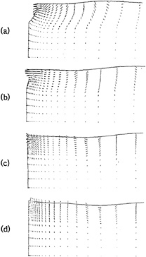
Fig.6 Velocity vectors on transverse sections at Fn=0.316 (a) x/L=0.84 (b) x/L=0.94 (c) x/L=1.00 A.P. (d) x/L=1.06
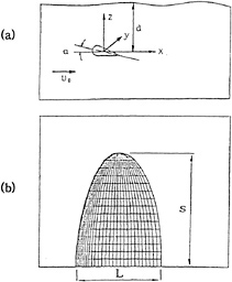
Fig.7 Coordinate system and elliptic span view of 3-D submerged hydrofoil
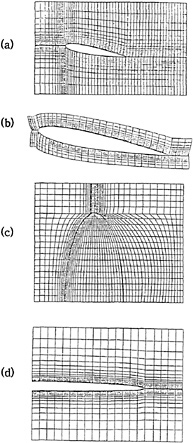
Fig.8 Grid view for case 2 (a) x-z plane (b) Closed-up view (c) x-y plane (d) y-z plane
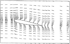
Fig.9 Velocity vector for case 1 (symmetric plane, j=3)

Fig. 10 Free-surface profile and velocity vectors on the three parallel surfaces of case 2 (a) j=3 (b) j=15 (c) j=20 (near tip)

Fig. 11 Free-surface profile and velocity vectors on the symmetric plane, j=3 (a) case 3 (b) case 4
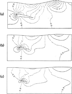
Fig. 12 Pressure contours for case 2 (a) j=3 (b) j=15 (c) j=18

Fig. 13 Pressure contours for cases 3 and 4 (a) case 3, j=3 (b) case 4, j=11


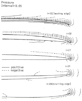

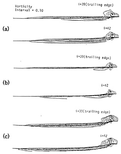
Fig. 18 Chordwise vorticity contours at i=39 and 42 (a) case 2 (b) case 3 (c) case 4
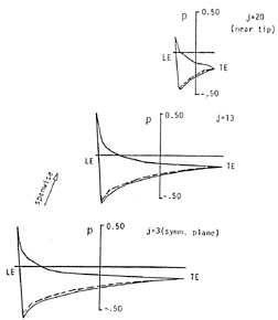
Fig.19 Comparison of spanwise pressure distribution on wing surface Lower;suction, upper;pressure (—; case 1, - - -; case 2)
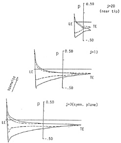
Fig.20 Comparison of spanwise pressure distribution on wing surface. Lower;suction, upper;pressure (—; case 2, - - -; case 3)

Fig.21 Comparison of spanwise pressure distribution on wing surface Lower;suction, upper;pressure (—; case 3, - - -;case 4)

Fig.22 Comparison of lift coefficients for cases 1, 2, 3, 4 and 5
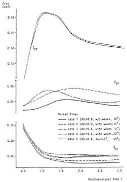
Fig.23 Comparison of drag coefficients for cases 1, 2, 3, 4 and 5
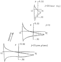
Fig.24 Comparison of spanwise pressure distribution on wing surface Lower;suction, upper;pressure (—;case 4, - - -;case5)

Fig.25 Spanwise lift distribution of port and starboard sides
DISCUSSION
by Dr. T.Hino, Ship Research Institute, Japan
The authors use two time-integration methods in solving the Navier-Stokes equations: one is the SIAF method and the other is the explicit method. In Figure 2, time history of drag coefficients shows that the two methods give different converged solutions. If the spatial discretizations of the two methods are identical, the solutions should converge to the same value. What causes the difference?
Author's Reply
In the calculation, the frictional drag is directly obtained by the difference of the velocities at the two points near the hull surface, and the pressure drag by the integration of the pressure on the hull surface. One of the numerical inconsistencies may be the different treatment of boundary conditions near the hull surface.
The explicit method has a very simple boundary condition by nature inside the hull surface. However, the implicit factorization method gives much more complicate boundary condition inside the hull surface in which the contravariant velocities are invoked to handle the boundary conditions. The reason of the difference can't be clearly explained, but it is certain that there is a numerical contradiction between the two applications.
DISCUSSION
by Professor K.Mori, Hiroshima University, Japan.
Owing to the introduction of the IAF scheme, you increased the time interval by four times. This may be okay for the momentum equations, but may not for the computation of free-surface elevation. Higher approximation should be introduced for the wave calculations also if you increase the time step.
Author's Reply
According to our results, the free-surface elevation is almost the same between the two methods even though authors increase the time interval by four times. One of the advantages in the present scheme is the reduction of the computational time with the similar results to the explicit ones. However, in order to get the improved free-surface, higher approximation and/or new boundary conditions at the downstream or lateral side may be necessary for the free-surface development.
DISCUSSION
by Dr. Y.T.Lee, David Taylor Model Basin
The grid systems used in this paper, particularly the one used for the Wigley case 74×29×19, are too coarse both in Y and Z directions. This implies that the solutions obtained are basically Euler solutions. The inconsistent results shown in Fig. 2 for drag coefficients at large time from two different approaches may be related to error in the viscous term.
Author's Reply
The grid system used in the computation is too coarse as you commented. In this connection, authors have an experience to calculate the full Navier-Stokes equations at two Reynolds numbers. One is 104 and the other 106. According to the calculated results, the effect of Reynolds number is obviously seen. It means that the coarse grid doesn't always give the results based on the Euler solutions. Authors agree that the coarse grid may be related to some errors in course of the long iterative procedure.
DISCUSSION
by Professor J.Feng, Penn State University
Four very simple questions:
-
Would the authors explain why a non-conservative formulation was chosen for convective terms instead of a conservative form?
-
A five-point differencing was used for viscous flux differencing. This leads to a penta-diagonal matrices, which are more expensive to solve than a tri-diagonal system form a three-point plus two half-point formulation.
-
Three dimensional ADI are not unconditional stable
-
A seemingly non-changing Ct/Cf/Cp is not a good criteria of convergence. In fact, Fig. 2 seems to suggest that the solutions are far from converging. At convergence, the explicit and the semi-explicit scheme should approach a common
-
numerical solution since they share the same right-hand terms. But more importantly, the fact that the two group of curves are flat and the different appears to imply numerical results will not converge easily or may even never converge at all.
Author's Reply
-
Non-conservative form has better stability property. The conservative form is dominantly used with compressible equations.
-
A five-point central differencings are used to increase the solution accuracy with a given number of grid points, thus resulting in block pentadiagonal systems. At points adjacent to the point of singularity or solid wall boundary, the three-point differencing formula are used for the first and second derivatives.
-
A three-level sweep scheme allows the spatial terms to be included efficiently in a spatially factored algorithm without upsetting the unconditional stability.
-
Please refer to the reply on the Hino question.
Numerical Prediction of Ship Generated Internal Waves in a Stratified Ocean at Supercritical Froude Numbers
M.P.Tulin, P.Wang, and Y.Yao
(University of California, Santa Barbara, USA)
ABSTRACT
Here we develop a non-linear theory for the solution of the near and intermediate internal wave field caused by a ship passing through a stratified ocean. The theory is mainly composed of a perturbation cross flow theory and is asymptotic to the case of very high supercritical ship speeds in the regime of greatest interest for modern ships, and to the case of small density differences. FEM is employed for numerical implementation.
Calculations have been carried out to distances from 10 to 80 ship lengths behind the stern for several speeds, F, and pycnocline distributions, ρ(z). The formation of a propagating trough followed by a crest, and successive waves has been found. A comparison of the predictions with experiments carried out in our laboratory, shows good agreement between measured and calculated wave patterns and amplitudes.
NOMENCLATURE
|
x, y, z |
: moving Cartesian coordinates |
|
s |
: path of the water particle |
|
ρ(z) |
: vertical density distribution |
|
ρ1 |
: density of the upper homogeneous layer |
|
ρ2 |
: density of the lower homogeneous layer |
|
Δρ |
: density difference, Δρ=ρ2−ρ1 |
|
H |
: depth of water |
|
h |
: mid depth of the pycnoclines |
|
δ |
: thickness of pycnoclines |
|
Us |
: ship speed |
|
L |
: ship length |
|
D |
: ship depth |
|
|
: scale parameter, |
|
FL |
: Froude number scaled with the ship length, |
|
Fh |
: densimetric Froude number scaled with h, |
|
|
: homogeneous velocity vector in x-y-z space, |
|
|
: perturbation velocity vector in y-z plane, |
|
|
: sum of homogeneous and perturbation velocity vectors in x-y-z space, |
|
q |
: water particle speed |
|
|
: potential of 3-D homogeneous flow |
|
ψ |
: stream function of 2-D perturbation flow |
|
|
: vorticity vector, |
|
|
: pressure gradient |
|
^ |
: denoting nondimensionalized variables |
|
Ni |
: high order Hermite shape functions, i=1, ..., 12 |
|
Hi |
: standard bilinear shape functions, i=1, .... 4 |
INTRODUCTION
The discovery that ships create internal waves when traveling in stratified water is due to Ekman (1904). In fjords and similar highly stratified water bodies ![]() , the surface disturbances due to the subsurface disturbances may be readily observed. Radar remote sensing makes ship internal waves even more readily detected, and has caused renewed interest in the subject. Internal waves are dispersive and the dispersion relation depends on the vertical density distribution and may be calculated from it The far field kinematical wave pattern due to a localized moving disturbance may also be predicted from the dispersion relations using ray methods, Keller and Munk (1970), or equivalent asymptotics, Yih(1990), Tulin & Miloh (1990). The latter, further, found an expression for the amplitudes in the far field, in terms of an amplitude function, following the technique introduced for ship waves by Havelock (1934).
, the surface disturbances due to the subsurface disturbances may be readily observed. Radar remote sensing makes ship internal waves even more readily detected, and has caused renewed interest in the subject. Internal waves are dispersive and the dispersion relation depends on the vertical density distribution and may be calculated from it The far field kinematical wave pattern due to a localized moving disturbance may also be predicted from the dispersion relations using ray methods, Keller and Munk (1970), or equivalent asymptotics, Yih(1990), Tulin & Miloh (1990). The latter, further, found an expression for the amplitudes in the far field, in terms of an amplitude function, following the technique introduced for ship waves by Havelock (1934).
The celerity of the first fundamental, and fastest, wave, c*, is approximately 30–50 cm/sec in both the ocean and fjords. The wave patterns depend upon Fh=Us/c*. The so-called dead-water phenomena resulting in greatly enhanced ship resistance occurs for Fh=O(1); for these speeds, the wave pattern is essentially transverse, see Miloh & Tulin (1988). However, the speed of modern ships is normally sufficiently high so that ![]() , and in this case the waves are solely divergent, within a half angle, β, where sinβ=1/Fh.
, and in this case the waves are solely divergent, within a half angle, β, where sinβ=1/Fh.
In the case of a two layer fluid, and for waves of small amplitude, wave fields may be calculated utilizing appropriate source-like singularities to represent bodies. This has been done: see, for example, Miloh, Tulin & Zilman(1992), where same examples of wave fields for different regimes in Fh are shown.
The specific calculation of the near field displacement patterns was first carried out by Tulin & Miloh (1990) using a shallow pycnocline (long wave) approximation. The resulting calculations revealed an upwelling in the near wake behind the ship, accompanied by negative deflections on either side, the triple lobe pattern. They have suggested that the far field has its origin in and results from the relaxation of the triple-lobe pattern, and may therefore be predicted from it.
Conceivably, suitably large forcing of the pycnoclines could result in the generation and propagation of soliton disturbances just outside the half angle, β. It would therefore be desireable to have available a theoretical method for the prediction of ship internal waves including non-linear terms.
In the present work we take advantage of the strongly divergent nature of the wave pattern for ![]() to develop a numerical calculation method for the theoretical prediction of both near and far field internal wave patterns for arbitrary vertical density distributions and for slender ships of arbitrary cross section, including the dominant nonlinear terms.
to develop a numerical calculation method for the theoretical prediction of both near and far field internal wave patterns for arbitrary vertical density distributions and for slender ships of arbitrary cross section, including the dominant nonlinear terms.
Very recently, Wong & Calisal (1993) have presented a numerical cross flow theory, with results. This interesting theory differs from that presented here in several respects : the forcing is calculated as part of the cross flow, whereas here the forcing is taken from the homogeneous flow; the density distribution corresponds to a two layer fluid. Their theory seems therefore most appropriate in the case of relatively shallow, sharp pycnoclines.
The validation of theory has been handicapped by a lack of systematic data. Therefore, Ma & Tulin (1992) carried out experiments on ship internal waves utilizing a small stratified tank and a small towed model of length, 45 cm. Longitudinal wave cuts at various transverse distances have been made for a spheroidal model, half submerged, over a range of Fh, both close to and much larger than unity, Ma (1993).
Here we describe the new theory and present specific calculations in four cases for which experimental data have been obtained in our laboratory. Satisfactory comparisons are made, so that the present method can be effectively used for the numerical study of ship internal waves, including non-linear effects.
The examples given here are for a simple spheroidal hull shape and simple pycnocline distributions, but the program created may be used for more general hull shapes and density distributions.
CROSS FLOW THEORY
We consider here an incompressible and inviscid fluid with a variation of density ρ in the vertical direction. The density profile is typified by a shallow layer of water with constant density ρ1 above, and an infinite depth of water with higher constant density ρ2 beneath, pycnoclines where the density changes continuously from ρ1 to ρ2. A ship with small ratio of draft D to length L passes above or through the pycnoclines, its speed Us is much larger than the limiting speed of internal waves, ![]() , as shown in figure 1. In these supercritical cases (densimetric Froude Number Fh= Us /c*≫1), the internal wave patterns generated are essentially divergent, the waves propagate in the the direction transverse to the ship' s direction, and the wave pattern is contained within a half angle to the ship's direction of sin−1(1/Fh). In a medium with small density differences, and for Fh≫1, the velocities in the near field of the ship can be composed of the sum of the homogeneous field, with no density gradients, and a perturbation field, representing the internal wave field, where the latter (and only the latter) is assumed two-dimensional in the cross flow plane, and becomes the entire disturbance in the far field.
, as shown in figure 1. In these supercritical cases (densimetric Froude Number Fh= Us /c*≫1), the internal wave patterns generated are essentially divergent, the waves propagate in the the direction transverse to the ship' s direction, and the wave pattern is contained within a half angle to the ship's direction of sin−1(1/Fh). In a medium with small density differences, and for Fh≫1, the velocities in the near field of the ship can be composed of the sum of the homogeneous field, with no density gradients, and a perturbation field, representing the internal wave field, where the latter (and only the latter) is assumed two-dimensional in the cross flow plane, and becomes the entire disturbance in the far field.
We consider the generation and propagation of these ship internal waves in a frame of reference stationary relative to the ship. In a coordinate system fixed in the moving ship, with the x-axis ![]() downstream, y-axis
downstream, y-axis ![]() transverse and z-axis
transverse and z-axis ![]() upward, see figure 1, the velocity field is decomposed, as discussed above, into:
upward, see figure 1, the velocity field is decomposed, as discussed above, into:
(1)
where,
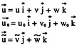
(2)
and (u0, v0, w0) is the homogeneous flow field with potential ![]() 0 driven by the passing ship, where it is usually but not necessarily appropriate to consider the free surface to be a rigid lid. This double model flow can be calculated by standard methods. In the specific calculations given here, we consider the flow past spheroids, so that the homogeneous ship flow is represented by a linear source distribution m(x) on the free surface, −L/2≤x≤L/2 :
0 driven by the passing ship, where it is usually but not necessarily appropriate to consider the free surface to be a rigid lid. This double model flow can be calculated by standard methods. In the specific calculations given here, we consider the flow past spheroids, so that the homogeneous ship flow is represented by a linear source distribution m(x) on the free surface, −L/2≤x≤L/2 :
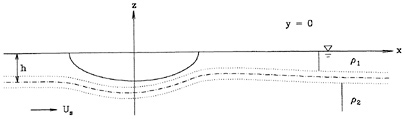
Figure 1 : A Stationary Flow Due to Ship Passing Over Pycnoclines, Actual Calculations. The Vertical Scale Has Been Stretched. (Δρ/ρ2=10−3, Fh=5, D/L=0.1, h/D=1, δ/h=0.4)
(3)
m(x)=−8πUs(D/L)2x (4)
The flow field, ![]() , causes the isopycnics to become inclined to the horizontal. Then, the pressure and density gradients interact to create vorticity in the region of stratification. This vorticity first creates a narrow region of displacements within the wake behind the ship, and these displacements relax to form internal waves propagating transversely.
, causes the isopycnics to become inclined to the horizontal. Then, the pressure and density gradients interact to create vorticity in the region of stratification. This vorticity first creates a narrow region of displacements within the wake behind the ship, and these displacements relax to form internal waves propagating transversely.
The vorticity arises in accord with Fridman's relation (Kochin et al, 1948), where the forcing is through the pressure term on the right,
(5)
where
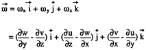
(6)
Since both the ship and the internal wave pattern are slender, ![]() in the near field, where
in the near field, where ![]() in the far field; for the same reason, the perturbations in u above are
in the far field; for the same reason, the perturbations in u above are ![]() and smaller than v,w. Therefore, from (6),
and smaller than v,w. Therefore, from (6), ![]()

(7)
Applying (5) in x direction, the first term of the LHS may be written in the steady case: ![]() , where q is the flow speed on the streamsurface. Within the same approximation, we obtain,
, where q is the flow speed on the streamsurface. Within the same approximation, we obtain,
(8)
The pressure can be expressed in terms of the velocity field through Euler's equation:
(9)
then (8) becomes,
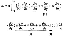
(10)
where [1] represents the horizontal inertial accelerations, [2] the vertical inertial accelerations, and [3] the gravitational acceleration.
The magnitude of these terms in the near field may be understood by introducing nondimensional variables appropriate to the near field:
(11)
then Eq (10) becomes,

(12)
The gradient ![]() is O(1), but
is O(1), but ![]() is in ratio to the former by the factor tan(α), where α is the tilt of the pycnoclines from the horizontal. Since FL is normally in the range 0.1∼0.3, the term
is in ratio to the former by the factor tan(α), where α is the tilt of the pycnoclines from the horizontal. Since FL is normally in the range 0.1∼0.3, the term ![]() dominates within the second bracket.
dominates within the second bracket.
In the y-z cross flow plane, we introduce a stream function ψ to represent the perturbation flow or the internal wave field ![]() , which satisfies,
, which satisfies,
(13)
then from Eq. (7), we deduce the Poisson Equation in nondimensional form, which governs the generation and oscillation of the internal waves in the cross flow plane, with the vorticity as its forcing term,
(14)
where,
(15)
Because the whole flow field is symmetric about the mid-line of the ship, or the x-axis, we take
the cross flow as a closed flow in half of the y-z plane with a continuous streamline of value zero on the whole boundary. Considering the fact that surface wave modes and internal wave modes are uncoupled and the amplitude ratio of these two wave systems is of order of Δρ/ρ2 (Phillips, 1967), we approximate the free surface as a rigid-lid. The infinite boundary in the y direction can be moved to a position where the leading internal wave has yet to arrive. The bottom boundary can also be taken where the disturbances have sufficiently decayed in depth.
The generation of vorticity and the deflection of the pycnoclines, or the oscillation of internal waves, are mutual and simultaneous, so Eqs (12) and (14) are coupled in a complex way. In the numerical simulation however, they can be decoupled by an iteration technique or simply by separating their calculation by an infinitesimal time interval. We choose the latter since the internal waves are long waves of steepness around one tenth and the velocity field changes very slowly. The calculation may be made by marching downstream since there is no upstream influence between the vorticity and the internal wave field.
In the x direction, the Lagrangian Method can be used to follow the fluid particles from one cross plane to another, resulting in pycnoclines in each new cross plane, and thus a three dimensional internal wave picture can be drawn. The starting cross plane is at x=x0, some distance before the bow of the ship, where the homogeneous flow field is still uniform and pycnoclines are still horizontal, as no vorticity has yet been generated.
In succeeding sections, the caps on nondimensional variables will be deleted for simplicity.
NUMERICAL IMPLEMENTATION
The physical problem discussed above can be described mathematically as an initial value problem in time, or in the x direction, which is solved by marching forward, plus successive boundary value problems in the y-z plane. Two corresponding computational domains are shown in figure 2.

Figure 2: Schematic Computational Domains
It can be seen in figure 2(b) that the breadth of the cross flow domain will continually increase after some distance along the x direction at x=xIR in view of the divergent property of internal waves. Bo is selected to allow a full depression under the ship; BF is the front of the transverse waves obtained from far field theory (Tulin & Miloh, 1990), and BI is a constant distance added on BF.
As discussed in the section above, velocity and vorticity fields can be solved separately at infinitesimal time intervals, or infinitesimal distances in the x direction. At the begining cross plane, x=x0, the vorticity is zero, the velocity field is taken from the homogeneous flow, ![]() ; the pycnoclines are horizontal with an imposed density profile, and then the first vorticity increment can be calculated, using Eq.(12), where
; the pycnoclines are horizontal with an imposed density profile, and then the first vorticity increment can be calculated, using Eq.(12), where ![]() . In the successive ith y-z plane, x=xi−1+Δx, the position of the pycnoclines is obtained by following fluid particles from the (i-1)th plane to the ith plane, where the distance the particles have travelled is Δs=q (Δx/Us); density gradients can also be calculated from the deflection of the pycnoclines, and the velocity field,
. In the successive ith y-z plane, x=xi−1+Δx, the position of the pycnoclines is obtained by following fluid particles from the (i-1)th plane to the ith plane, where the distance the particles have travelled is Δs=q (Δx/Us); density gradients can also be calculated from the deflection of the pycnoclines, and the velocity field, ![]() , is obtained by solving the Poisson equation, Eq.(14), with vorticity integrated from the previous section as the forcing, Eq (12), wherein
, is obtained by solving the Poisson equation, Eq.(14), with vorticity integrated from the previous section as the forcing, Eq (12), wherein ![]() . Marching through a sufficient distance after the ship, first a triple-lobed wake displacement pattern, and subsequently a three dimensional dispersive internal wave pattern appears. For Δx reasonably small, a high accuracy of simulation can be achieved.
. Marching through a sufficient distance after the ship, first a triple-lobed wake displacement pattern, and subsequently a three dimensional dispersive internal wave pattern appears. For Δx reasonably small, a high accuracy of simulation can be achieved.
The essence of the current theory is the perturbation cross flow in the y-z plane governed by the Poisson Equation, with vorticity penetrating the plane as its forcing. So the crux of the numerical implementation is in solving a two dimensional boundary value problem with an elliptic P.D.E. as its field equation, and Dirichlet conditions around the whole boundary.
Finite Difference and Finite Element Methods are two numerical techniques available for this problem, but the latter is more suited to modelling curved boundaries, like the ship hull boundary, and when non-uniform gridding is used. To allow for a large field simulation which consumes considerable CPU resources, a graded spatial discretization is preferred, and refined meshes in the z-direction are used within the pycnoclines, where the density of the fluid changes rapidly; the size of the meshs which are away from the pycnoclines increase gradually upward or downward. In the y-direction, the size of the mesh increases gradually proceeding outwards since internal waves propagate outwards with the longest wave in the front. To catch the interfacial movement of the pycnoclines, the easiest way is by always following their particles, so the grids have to be on the wavy changing pycnoclines. For all these reasons, the Finite Element Method is employed for the current task.
In the classical Galerkin finite element method, the weight functions are chosen to be equal to the element shape functions. A discrete analog of the continuous physical system, which is governed by the Poisson equation, is given by,
(16)
where Ni are the weight functions; Ω represents the whole calculation domain in the y-z plane. Integrating by parts to reduce the second order
derivatives to the first order, and expressing Eq.(16) as a finite sum of integrations on piecewise continuous elements, we obtain,

(17)
where Ωe is the integration domain in each element in the y-z plane, Bi, i=1, 2, …, 5, is the boundary of the computational domain as indicated in figure 2(c), and ∂Ωe is the integration boundary of elements on those boundaries; Ψ(e) and (ωx)(e) are the interpolated stream function and vorticity distribution variables in each element represented by linear interpolation of their discrete values on element nodes.
The selection of the type of element is very important for the success of the current numerical approach. We follow particles in the x direction by their velocity to complete a stationary three dimensional wave pattern. And vorticity involves velocity derivatives. So the accurate approximation of first and second order derivatives of the stream function is crucial in the numerical simulation of ship generated internal waves. We choose a high order Hermite element, because it has both the variable and its first order partial derivative all as unknowns, and allows the second order derivatives, which do not occur in the governing equation, to be differentiated based on the velocity field which is interpolated by a linear combination of its discrete nodal values.
Considering both accuracy and computer time expenses, and comparing two polynomial bases for triangles and quadrilaterals, Eq (18) and (19), four node cubic Hermite elements are employed to partition the computational domain into finite elements. This allows the continuity condition to be satisfied on nodes of elements. Continuity of the stream function and tangential velocities across element boundaries are also preserved.
{P}3={1 ξ η ξ2 ξη η2 ξ3 ξ2η ξη2 η3} (18)
{P}4={1 ξ η ξ2 ξη η2 ξ3 ξ2η ξη2 η3 ξ3η η3 ξ3η ξη3} (19)
The stream function in each element is thus interpolated by a linear combination of its nodal values using 4-node cubic Hermite shape functions Ni (i=1, …, 12),
(20)
Element coordinates and all the other variable functions, like velocity, density and vorticity, are interpolated using the standard bilinear shape functions Hi (i=1, …, 4) that is,
(21)
Variable derivatives are carried out based on interpolated variable functions and transformed from local (ξ, η) to a general (y, z) coordinate system by the Jacobian operator.
It should also be mentioned that all variable derivatives, except velocity, calculated on grids except at corners of the domain are averaged on the surrounding elements with equal weight
The cubic Hermite shape functions Ni and the bilinear shape functions Hi, and their first order partial derivatives ∂Ni/∂ξ, ∂Ni/∂η and ∂Hi/∂ξ, ∂Hi/∂η are available in the literature. With careful geometrical treatment of the physical domain and application of standard procedures in FEM, the stream function and velocity field can be solved together with sufficient accuracy.
We divide the y-z cross flow domain Ω into three parts, Ω1, Ω2, and Ω3, as shown in figure 2(c). The first part, Ω1, like a stream tube, includes all pycnoclines and is bounded by upper and lower interfaces with two constant density layers. The second part, Ω2, is the region in the upper layer and is near the boundary of the ship, where the mesh construction is a little harder than in the other two parts. The third part Ω3 represents the remaining part of the whole domain, including the layer beneath the pycnoclines and the right part of the upper layer. In Ω2 and Ω3, the vorticity is equal to zero, and no fluid particles need to be followed from one section to another.
In Ω1, one big stream tube is divided into multiple smaller ones, along which elements are distributed with neighboring segments being near-orthogonal to the streamlines, or the pycnoclines, as shown in figure 3. The element breadth increases gradually in the outflow direction.
Near the ship boundary, high curvatures are involved including two singular points. Generalized coordinates are normally more suitable for this kind of boundary. But here a band of the computational domain is predetermined by the physical flow, characterized by the oscillation of pycnoclines, the grid generation cannot be done automatically in the whole computational domain by algebraic mapping or by solving partial differential equations. To avoid complex manipulations or manual intervention during grid generation, a simpler technique is used in Ω2 at the cost of local element distortion near the

Figure 3 : On the Left, an Example of Grid Distribution in y-z Cross Plane, the Blank Part on Left-Upper Corner Represents a Quarter of a Section of a Double Hull Ship. On the Right, an Example of a Vertical Density Distribution.
ship boundary. This has little effect on the internal wave calculation.
In Ω3, meshes are formed comparatively free of any restrictions, and stretching out in the y direction and in the upward or downward direction within the upper and lower layers.
An example of grid generation is shown in figure 3. It can be seen that more grids are concentrated in the left part in the pycnoclines, whereas in the right and lower part of the domain, the mesh distribution is quite loose. It is reasonable to expect that the efficiency of the computation can be even more enhanced, by using a split-time technique, or a split-marching technique for the stationary flow; however this technique has not been implemented in the current stage.
RESULTS & DISCUSSION
The numerical code developed based on the above theory and computational techniques has been tested with regard both to the finite element solution of the Poisson equation, and the convergence of wave amplitudes for different marching steps in the x direction.
As a test flow, we consider a simple closed flow with a stream function,
ψ=sin(kyy) sin(kzz) (22)
where,
![]() n, m=1, 2, (23)
n, m=1, 2, (23)
B and H are the breadth and height of the physical domain, so ψ=0 on the entire boundary.
The velocity field for this stream function is,
(24)
An x component of vorticity exists within the whole flow field, and its value can be calculated directly from the known stream function, Eq (22),
![]()
=[(ky)2+(kz)2] sinkyy sinkzz (25)
We do the inverse problem numerically using our code, and compare the velocity field, solved from the Poisson equation, with the exact solution given in Eq (24). High resolution is achieved with 8 to 12 grids distributed uniformly in a half wave length, see figure 4.
In the x direction, as far as proper marching steps are concerned, the convergence test is carried out in the region from upstream ![]() to midship
to midship ![]() , where a big depression always occurs, with a larger displacement than elsewhere. A range of
, where a big depression always occurs, with a larger displacement than elsewhere. A range of ![]() from 0.005 to 0.05 was tested, and the wave amplitude and vorticity converge very well when
from 0.005 to 0.05 was tested, and the wave amplitude and vorticity converge very well when ![]() is less than 0.025, see figure 5; the errors relative to
is less than 0.025, see figure 5; the errors relative to ![]() are shown in table 1.
are shown in table 1.
Table 1 : Convergence Test—Relative Errors
|
|
Δη/η0.005 |
Δωx/(ωx)0.005 |
|
0.01 |
0.14% |
0.75% |
|
0.025 |
0.38% |
4% |
|
0.05 |
0.77% |
10% |
With the confidence obtained so far, we did a series of calculations with the physical conditions

Figure 4 : Numerical Test of the Finite Element Solution of the Poisson Eq. B=H=1.2, Velocities at Five Equally Spaced Positions of z (for v) & y for (for w) Are Compared. Left, n=m=1; Right, n=m=2

Figure 5 : Convergence Test for Marching Steps in the x Direction, ![]() . Three Bunches of Lines in Each Plot Correspond to Upper, Mid and Lower Interfaces. (F=4.76, D/L=0.097, h/D=1.28, δ/h=0.42, Δρ/ρ=0.0036)
. Three Bunches of Lines in Each Plot Correspond to Upper, Mid and Lower Interfaces. (F=4.76, D/L=0.097, h/D=1.28, δ/h=0.42, Δρ/ρ=0.0036)
listed in table 2, selected from tank experiments carried out in our laboratory; the case numbers are the same as used in the experiments.
Table 2: Physical Conditions of the Numerical Simulations (D/L=0.097)
|
Case No. |
h/D |
δ/D |
Δρ/ρ2 |
Fh |
|
41(c) |
1.28 |
0.54 |
0.0034 |
10. |
|
41(b) |
1.28 |
0.54 |
0.0034 |
4.8 |
|
28(b) |
0.96 |
0.29 |
0.0036 |
5.9 |
|
25(c) |
0.78 |
0.39 |
0.0041 |
6.5 |
An internal wave field as long as 80 ship lengths is simulated for case 41(c), figure 6(a) & (b),

Figure 6: Ship Internal Waves, Case 41(c), the Darkened Line Is the Cut for Triple Lobe. (a) Near and Intermediate Field; (b) Near Field, Blown up from (a).
which covers the near and intermediate internal wave field. It can be clearly seen that: a big displacement appears just under the ship; and starting immediately after the ship, a central peak accumulates gradually which separates and pulls up the down lobe until a typical triple-lobe pattern in the transverse direction forms; then, this deformation relaxes and produces dispersive waves which propagate outwards, with the longest waves in the front.
The kinematic wave pattern, represented by the phase lines corresponding to crests and troughs, has been compared with far field theory (Tulin & Miloh, 1990), and very good agreement is obtained, as shown in figure 7.
Occuring one and a half ship lengths after the stern of the ship, case 41c, where the centerline amplitude reaches its peak, a triple-lobe pattern with a sharp peak and two shallow troughs appears as shown in figure 8(a); its vertical velocities are shown in figure 8(b), which, with a little shift, is similar to the triple-lobe distribution, and has an almost zero velocity at the central point as intended. It was suggested by Tulin & Miloh (1990) that the far field internal wave pattern may be calculated upon the assumption that the far field wave pattern originates from the initial conditions represented in the triple lobed pattern. In that case, they showed that the entire far field may be represented by a complex amplitude function, which is readily calculated from a Fourier transform of the triple lobed pattern, amplitudes and velocities.
This calculation has been carried out here, see figure 9. The real part of the transform of the triple-lobe amplitudes, centers at kh around one and decreases slowly in each direction, case 41c; the imaginary part, originating from the vertical velocities in the triple-lobe pattern, has an infinite value at kh equal to zero and decreases fast when kh increases. The modulus of these two parts composes the amplitude function which can be used together with the far field kinematic pattern to represent the far field internal wave field.
In figure 10, downstream wave cuts at increasing transverse distance, y/D, are shown from two different calculations together with experimental data: the current direct numerical calculation, and the far field calculation using the calculated amplitude function. We get very good agreement between the two kinds of calculations, and generally good agreement with the experimental data.
More simulations are carried out for a densimetric Froude number around five and for different depths of pycnoclines. Results are shown from figure 7 to figure 10. It is seen that, very good agreement is also obtained for case 41(b) between current direct calculation and the calculation using the far field theory for both the kinematic wave pattern and wave amplitudes. With the success of the calculation of the amplitude function and the confirmation of the far field theory, in the case 28(b) and 25(c) we halted the direct calculation at the triple-lobe pattern, and then calculated the amplitude function, used it to predict the far field internal wave pattern using the far field theory.
A detailed comparison of the results is shown in Figure 10(a) to (d). In 10(a) and (b) very good agreement is seen between the present numerical far field calculations (–·–) and predictions made from the analytical theory of Tulin and Miloh based on amplitude functions computed from triple-lobed patterns calculated numerically using the present theory (.......). This agreement suggests that


Figure 9 : Far Field Amplitude Functions.
these detailed numerical calculations need only be carried out in the near field aft to the triple-lobe, providing that the waves are sufficiently small.
The experimental results (—) shown for comparison have been obtained in a small stratified tank using a towed model 45cm long (Ma & Tulin, 1992). The effects of the turbulent wake of the model are evident in the roughness of the wave patterns close to the model track and sufficiently aft The amplitudes found in the experiments and predicted theoretically are, in general, comparable — there certainly exists no major discrepancies in magnitudes, although a tendancy for theory to underpredict seems present; it must be kept in mind that the turbulent wake is not modeled here. In general, the agreement improves for cuts at the center of the larger transverse distances. A comparison of both theory and experimental measurements at much larger scales would be highly desireable.
A kh-map is shown in figure 11, in the case of 41b, which gives a clear view of the distribution of wave lengths in the patterns, and is helpful when far field wave amplitudes are analyzed using the amplitude function.
The CPU time needed for calculation in the near field to the triple-lobe pattern is only around 265 seconds, and for far field calculation to 80 ship lengths in case 41c, 371 minutes. All these calculations have been carried out on an IBM 9000.
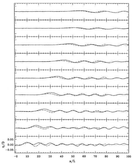
Figure 10(a): Longitudinal Wave Cuts at Transverse Distances from the Ship, Case 41c, from y/D=4.35 to y/D=40.35 in intervals of Δ y/D=4.5, Where —, Experimental Data, –·–, Direct Calculation Using Current Theory, ·······, Results From Far Field Theory Using Triple-Lobe Pattern From Direct Calculation

Figure 10(b) : Longitudinal Wave Cuts at Transverse Distances from the Ship, Case 41b, from y/D=4.35 to y/D=40.35 in intervals of Δ y/D=4.5, Where —, Experimental Data, –·–, Direct Calculation Using Current Theory, ·······, Results From Far Field Theory Using Triple-Lobe Pattern From Direct Calculation


Figure 11: a Typical kh-map of the Far Field of Ship Internal Waves Showing the Distribution of Wave Lengths in Wave Pattern and in Space
SUMMARY & CONCLUSIONS
A numerical method has been developed which is appropriate for slender bodies of arbitrary cross section traveling in a stratified ocean at sufficiently large densimetric Froude numbers, Fh ≫1.
This method assumes an inviscid flow field composed of a double model flow about the ship in homogeneous water plus a perturbation flow slowly varying in the x direction and therefore 2D in the cross flow plane. The 2D cross flow is described by the Poisson equation for the cross flow stream function, where the forcing is provided by the down stream vorticity, induced by deflections of the pycnoclines. The resulting solution satisfies the boundary conditions everywhere on the ship hull. The vorticity is calculated by a marching procedure, using an algorithm based on Fridman's Equation.
The method is applicable to arbitrary density profiles in depth and to arbitrary ship cross sections, and is non-linear in the cross flow plane and allows the propagation of solitons, none of which are generated in the examples given here.
The numerical method utilizes higher order Hermite finite elements and has been convergence tested.
Total calculations have been made for four cases for which small model experimental data on
the far field wave pattern exist. These were taken in our own laboratory.
The present computational method predicts a far field kinematical pattern in very good agreement with the predictions of analytical far field theory.
The computations show the development in the near field of a narrow pattern of deflections behind the ship, arising from the initial reaction of the pycnoclines to the depression by the ship hull. These deflections in the wake on the ship track, are upwards and reach a peak behind the ship, at which station the cross section of the depression pattern is upwards in the center and downwards on either side. The triple lobe pattern was originally discovered by Tulin & Miloh, 1990.
Far field amplitudes deduced from the analytic theory of Tulin & Miloh, using an amplitude function calculated from the triple lobe pattern computed here, are in very good agreement with the far field fully numerical calculations.
The results found here thus tend to confirm the triple lobe pattern as the source of initiation of the far field wave pattern. This places an emphasis on the calculation of the near field, and reduces the computing time by orders of magnitude.
The magnitude of computed wave amplitudes are in good general agreement with our experimental results, with same tendency for theory to underpredict, and for detailed comparisons to improve with increasing transverse distance from the ship.
Considering the influence which the turbulent wake might be expected to have on the flow in the direct wake of the ship, the agreement between small scale theory and these numerical predictions must be regarded as very good.
Additional comparisons with large scale experiments would be highly desireable.
ACKNOWLEDGEMENT
The authors are grateful for support from the Office of Naval Research, Ocean Technology Program, directed by Dr. Thomas Swean.
REFERENCES
Ekman, V.W., 1904. On Dead Water. The Norwegian North Polar Expedition 1893–1896, vol. V, Ch. XV, Christiania
Havelock, T.H. “The Collected Papers of Sir Thomas Havelock on HYDRODYNAMICS,” ONR/ACR-103, pp. 377–389
Keller, J.B. & Munk, W.H., 1970, “Internal Wave Wakes of a Body in a Stratified Fluid”, Physics of Fluid, Vol. 13, pp.1425–1431
Kochin, N.E., Kibel, I.A. & Roze, N.V., “Theoretical Hydromechanics,” 1948
Ma, H & Tulin, M.P., 1993. “Experimental Study of Ship Internal Waves : The Supersonic Case”, Journal of OMAE , Vol. 115, No.1, pp. 16–22.
Ma, H. , 1993. Dissertation, OEL, UCSB
Miloh, T. & Tulin, M.P., 1988. “a Theory of Dead Water Phenomena,” Proc. of the 17th Symposium on Naval Hydrodynamics, National Academy Press, 1988
Miloh, T., Tulin, M.P. & Zilman, G., 1992. “Dead-Water Effects of a Ship Moving in Stratified Seas”, Proc. of the 11th Intl Conf. on OMAE, 1992, Vol I, Part A, pp. 59–67
Phillips, O.M., Dynamics of the Upper Ocean, Cambridge, 1969.
Tulin, M.P. & Miloh, T., 1990. “Ship Internal Waves in a Shallow Thermocline: the Supersonic Case ”, Proc. of the 18th Symposium on Naval Hydrodynamics, National Academy Press, 1990
Wong, H.L. & Calisal S.M., 1992. “Waves Generated by a Ship Travelling in Stratified Water,” Proc. of the 3rd Intl. Offshore & Polar Engr. Conference, 1993
Yih, C.S., “Patterns of Ship Waves,” Engineering Science, Fluid Dynamics, World Scientific Publishers, 1990.


