Displacement Thickness of a Thick 3-D Boundary Layer
L.Landweber, A.Shahshahan, and R.A.Black
(University of Iowa and Loras College, USA)
ABSTRACT
Thin-boundary-layer solutions for displacement thickness were published in the fifty's. More recently, semi-empirical methods of computing displacement thickness were developed in connection with interactive methods of computing viscous flows about bodies. In the present work, the determination of the displacement thickness is recognized as a member of the class of “ill-posed problems” (IPP), in which small or random errors in the data defining a problem result in much larger errors in its solution. Otherwise, the displacement thickness of a given viscous flow can be well-defined mathematically by generalizing the thinboundary-layer solution. Rational solutions can then be obtained by applying the suggestions for controlling growth of errors given in the IPP literature.
The theory assumes that, exterior to a boundary layer, the flow is irrotational, that this irrotational flow can be continued into the boundary-layer region, and that this flow is singularity-free in that region. That is accomplished by means of a Fredholm integral equation of the first kind which, appropriately is a classical example of an IPP. The procedure is illustrated by applying it to a Wigley form.
INTRODUCTION
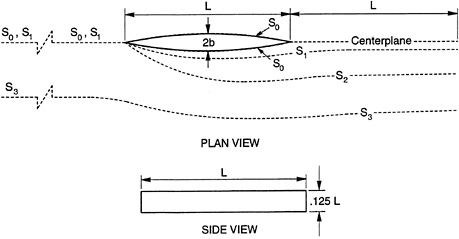
We suppose that a given double body of a ship form is at rest in a uniform stream U∞ of an incompressible fluid parallel to its centerplane, and that the vector velocity field v of the mean flow within the boundary layer and wake (BLW) of the ship form is known. Outside the BLW, we assume that the mean flow v is irrotational and coincides there, with a small error, with an irrotational vector V which may be continued as an irrotational velocity field V into the BLW. Let S3 be a member of the family of viscous-flow stream surfaces, lying exterior to the BLW, of which the body itself, S0 is the defining member. Then S3 also defines a different family of irrotational flow stream surfaces of V extending into BLW. The displacement-thickness surface S1 is defined as that member of the latter family which satisfies the flux condition that the flux of v between S0 and S3 is equal to the flux of V between S1 and S3. See Fig. 1.
If S2 is another surface, not necessarily a stream surface, but closer to the edge of BLW, S2 may replace S3 in the above definition of S, since we assume v=V between S2 and S3. The above definition implicitly assumes that V is singularity-free in the space between S1 and S2, except for a surface distribution on the centerplane of the wake. If that condition is not satisfied, then an exact solution for S 1 does not exist, although useful, approximate solutions may be found.
If the body has a well-defined stagnation point, the dividing streamline would be, by symmetry, a straight line, generating the given body in the viscous flow and S1 in the irrotational flow. This is seen to satisfy the flux condition, since, far upstream, the velocity fields of v between S0 and S3 and of V between S1 and S3, coincide. See Fig. 1.
Moore [1] and Lighthill [2] have treated the present subject for thin boundary layers. Both defined the displacement-thickness surface S1 as a stream surface, but neither introduced a flux condition. Moore terminated his analysis with a first-order partial differential equation (PDE) for the displacement thickness, derived from the streamsurface condition, the equations of continuity, and the thin boundary-layer approximations. Lighthill rederived Moore's equations, but also obtained explicit solutions for the displacement thickness and the equivalent source distribution on the body surface. Lighthill assumed that the stream surface of V which passes through the stagnation point(s) is the displacement-thickness surface. This assumption which is also made in the present work, can be
justified for symmetric flows about double models without a free surface, because then a free-surface boundary layer and wavebreaking are not present ahead of the bow and the stagnation points are well-defined.
In Stern, Yoo and Patel [3] an interactive method of computing the viscous flow about a 3-D body, involving displacement thickness, was developed. Beginning with an assumed first approximation, a succession of displacement bodies and the corresponding irrotational- and viscous-flow fields were computed iteratively. In that work, each transverse section of the S1-surface was assumed to be an ellipse of dimensions satisfying approximately a mean, local flux condition. Nevertheless, their viscous-flow results were in good agreement with experimental data and those computed by a large-domain method.
At the request of Fred Stern (FS), the present work was undertaken by Landweber (LL). It will be seen that an important phase of the project is the calculation of the continued irrotational flow into the boundary layer and wake (BLW). For that purpose, a method using a Fredholm integral equation of the first kind for determining the source distribution on the surface of the body equivalent to the displacement effect of the boundary layer, was proposed by LL and FS assigned an M.S. candidate, RA Black, to work with LL on the validation of the procedure. After verifying that the equivalent source distributions could be obtained with sufficient accuracy, the next step was to calculate the irrotational velocity field of the sources. For that purpose, a complicated Hess-Smith computer program [4] for the velocity field of a source distribution of constant strength on a flat quadrilateral panel was available; but, by transforming the integrals to ones over the centerplane of the body the projected panels became rectangular, and the integrals could be expressed more simply in closed form in terms of elementary functions. Since these results may be new and useful, they will be presented here.
Equivalent source distributions are of interest not only for calculating the effects of waves on the boundary layer of a ship, but also for the effects of the boundary layer on the wavemaking of a ship form. This was shown for the Weinblum very thin form by Kang [5] and by Shahshahan and Landweber [6] for the Wigley form, both using equivalent centerplane distributions. It will be of interest to calculate the wave-making resistance of the Wigley form using the present results for the equivalent source distribution on the body surface, although this is not done in the present work.
Here we shall derive a generalized version of Moore's partial differential equation, without applying the thin-boundary-layer approximations. Since the only application planned was to the Wigley form, it seemed most convenient to work in rectangular Cartesian coordinates, although the generalized PDE had also been derived in nonorthogonal coordinates. The PDE was then solved by a method of finite differences, using a method suggested by Lax [7].
The plan of the present work is as follows:
-
Obtain a source distribution on the body surface y0 and the centerplane of the wake as the numerical solution of an integral equation of the first kind, using given data for the viscous-flow velocity field exterior but close to the edge of the boundary layer.
-
Apply that source distribution to compute the irrotational velocity field within the boundary layer and wake.
-
Apply the irrotational and viscous-flow velocity fields to compute the auxiliary displacement thicknesses α and β defined in Eq. (4). Also compute the derivatives of the velocity components at y0 occurring in Eq. (11).
-
Use method of finite differences to solve the partial differential equation (10) and (11) for δ1, defined in (4).
NATURE OF THE PROBLEM
Let us suppose that the edge of the BLW is defined by a contour surface at H=0.990 H∞, where H denotes the total head at the contour and H∞ the asymptotic value of the total head at great distances upstream or lateral to the body. Had H been defined by H=0.995 H∞, the edge of the BLW would be much farther from the centerplane and the error in assuming irrotational flow there would be reduced, but the accuracy of analytical continuation of that flow into the BLW region would be greatly diminished. Indeed, the procedure adopted here to continue the potential flow strongly suggests that the present work is on an “ill-posed problem,” in which small or random errors in the data defining a problem results in much larger errors in its solution, as defined by Tikhonov and Arsenin in[8].
The simplest case of an ill-posed problem is a set of linear, algebraic equations, Ax=b, where A is a matrix and x and b are vectors. This has an exact solution when the A is nonsingular (i.e. its determinant is not zero); but if A is nearly singular and the right member is subject to errors, the resulting errors in the solution would be amplified. Another classic case is the Fredholm integral equation of the first kind, which, in general does not
have an exact solution. If discretized by means of a quadrature formula, this case reduces to the previous one, yielding approximate solutions with possibly large errors.
The literature on ill-posed problems presented in [8] indicates that it is possible to get useful results by use of supplementary information, such as requiring smoothness of the solution, or by a process called “regularization” developed by Tikhonov in a series of six papers from 1963–65. The method of constructing approximate solutions is called the “regularization method.” This method requires finding or constructing a regularization operator which transforms the equation of the ill-posed problem so that approximate, stable solutions (i.e. solutions without error amplification) could be found. Construction of this operator appears to be a difficult task. Twelve years prior to Tikhonov's work on this concept, Landweber [9] had shown that the integral operator of an integral equation of the first kind transforms the equation into one with a symmetric kernel with which stronger convergence properties of an iteration formula could be proved. In that sense, the original operator of the ill-posed problem could serve as a regularization operator. Reference [9] is not included among the 221 papers listed in the Bibliography of [8].
FORMULATIONS OF STREAM-SURFACE EQUATIONS
The equation of continuity and the stream-surface equation will now be applied to generalize the thin boundary-layer treatments of Moore [1] and Lighthill [2] for a double ship form. Let (x,y,z) denote a rectangular Cartesian coordinate system with origin at the forward stagnation point, the x-axis parallel to the uniform stream and positive in the downstream direction, with the x- and z-axes lying in the vertical centerplane, and the z-axis positive upwards. Let (u,v,w) and (U,V,W) denote the components of v and V. Also let y=y0(x,z), y =y1(x,z), y=y2(x,z) denote the equations of a given hull surface S0, its displacement thickness surface S1 and a surface S2, near but exterior to BLW, respectively. At S0, the velocity components will be designated by
where ![]() ,
, ![]() ,
, ![]() denote unit vectors in the x,y,z-directions; and there, by the nonslip condition,
denote unit vectors in the x,y,z-directions; and there, by the nonslip condition,
(1)
Since V is irrotational, we have
![]() ×V=0,
×V=0, ![]() 2V=0 (2)
2V=0 (2)
and on S2, we assume
u2=U2,v2=V2,w2=W2 (3)
We also define the three auxiliary displacement thicknesses

(4)
These definitions of α and β assume that V and W are singularity-free for y0≤y≤y2. We also assume that α and β are of the order O(δ1) for a body of unit length.
The equations of continuity for v and V are
(5)
Then, integrating equations (5) with respect to y from y0 to y2, taking their difference and applying (1) and (3), we obtain
(6)
or, applying (4) and the Leibnitz rule for the derivative of an integral, we get
V0=U∞(αx+βz)+U0y0x+W0y0z (7)
where subscripts x and z denote partial differentiation with respect to the indicated variable.
The condition that the y1 surface be a stream surface is

(8)
where
V1=V(x,y1,z)
Since the y1 surface is unknown, we transfer (8) to the known surface y0 by means of the Taylor expansions

which, substituted into (8), gives

(9)
By substituting for V0 from (7), replacing Vy by-UX-WZ, Vyy by -VXX-VZZ and neglecting the ![]() terms, we obtain
terms, we obtain
(Px+Qz)0=R(x,z,δ1) (10)
where
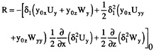
(11)
and
P(x,z)=Uδ1−U∞α, Q(x,z)=Wδ1−U∞β
Here the left member is clearly of order 0(δ1). The first term of the right member also seems to be of order 0( δ1); but, as will be seen, computationally, its effect is that of a second-order term, and the remaining terms are of even higher order, at least for the Wigley form. We also observe that the homogeneous form of (11) when R=0, is essentially Moore's partial differential equation expressed in rectangular, Cartesian coordinates.
CONTINUATION OF OUTER IRROTATIONAL FLOW INTO BOUNDARY LAYER
Source Distribution on Body
Let Φ denote the velocity potential of the irrotational flow about the displacement body in a uniform stream and ![]() that of the disturbance potential. Then
that of the disturbance potential. Then
Φ=![]() +U∞x (12)
+U∞x (12)
and V, the y-component of V, is given by ![]() in the exterior of BLW according to (3). Since v is given, grad Φ is known on y2, but we shall require only V.
in the exterior of BLW according to (3). Since v is given, grad Φ is known on y2, but we shall require only V.
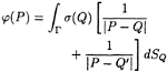
We assume that potential flow ![]() is generated by a source distribution σ(xQ,zQ) on the hull surface yo and the centerplane of the wake may be written as
is generated by a source distribution σ(xQ,zQ) on the hull surface yo and the centerplane of the wake may be written as
(13)
where P denotes a point exterior to BLW and rPQ the distance between points P and Q,
Then, differentiating with respect to yP, we obtain

(14)
a Fredholm integral equation of the first kind.
By applying a quadrature formula of order N, (14) can be reduced to a set of N linear equations for σQ, i=1, 2…N which can be solved by a computer using available software. It is well known, however, that small changes in VP in (14) may cause large changes in σQ when the set of linear equations is nearly singular; i.e. when the determinant of the coefficients is nearly zero. This was verified in several test cases in which the velocity was computed at points exterior to a body due to an assumed source distribution on the surface of the
body. Then the relation between the source distribution and the velocity was treated as an integral equation of the first kind to try to recover the source distribution. This preliminary work yielded the conclusions that double precision should be used and that an iteration formula for integral equations of the first kind due to Landweber [9] yielded useful results even when a linear-equation solver had failed.
In order to derive the convergence properties of the iteration formula of [9], the original kernel of the integral equation was transformed into a symmetric one. Since that requires a large number of additional integrations for a 3-D problem, it is customary to assume that the iteration formula with the original kernel would have similar convergence properties. In general, integral equations of the first kind do not have exact solutions, but a sequence of approximate solutions can be found which converges in the mean, i.e. the integral of squares of the errors becomes very small. In practice, the successive approximations are monitored so that the sequence can be stopped when the errors are as small as desired, or, in case of initial convergence and then divergence, when the errors begin to grow. An important difference between the preliminary tests of the integral equation method on a Wigley form and a calculation of the unknown function is that, in the former case, the exact solution was known, and, in the latter case, the existence of a solution was uncertain.
The equation of the Wigley form for which results were computed is
(15)
Here the body length is L=2ℓ, b is half the beam and h is the draft. We take L=1, b=0.10ℓ and h =0.125ℓ. The limits of integration of the integral in (14) are taken to extend over the double body and over the centerplane of the wake for an additional ship length L and for z varying from −h to +h. The integral in (14) may then be written as
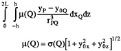
(16)
Since μ(Q) is the same in the four quadrants of a transverse section, the four terms with yQ≠0(0<x<L) and the two terms with yQ=0 (L≤x≤2L) can be collected into a single expression for integration over the first quadrant of Q's for any point P in the first quadrant,
(17)
where
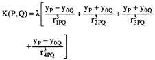
with λ=1 when yQ≠0 and λ=1/2 when yQ=0, and
The integral in (17) may be interpreted as extending over the centerplane; although y0(x,z) is not replaced by zero, i.e. the unknown source distribution is still on the body. Adopting the iteration formula of [9], but with the original kernel, we obtain

(18)
Here P and Q have the coordinates (xP, yP, zP) and (XQ,Y0(xQ,ZQ),ZQ), and VP and the integral are functions of the coordinates of P. Hence, in the present coordinate system we must take (xp,zp) and (xQ, zQ) as the same array of numbers and interpret the iteration as giving a corrected source distribution at the same points Q. “C” is a constant, selected so as to accelerate the convergence. To initiate the iteration, the selected value of ![]() , suggested by slender-body theory is
, suggested by slender-body theory is

(19)
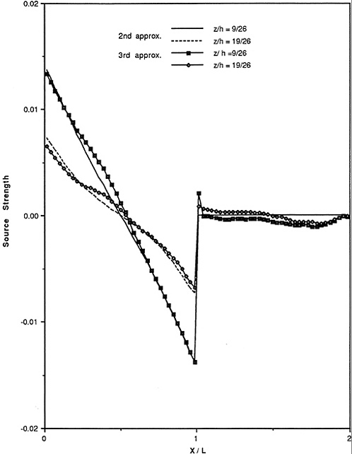
Equation (18), discretized by the panel method of the next section, becomes
(20)
results, obtained with 70 values of x and 13 values of z, with C=1, are shown in Figures 2, 3a and 3b.
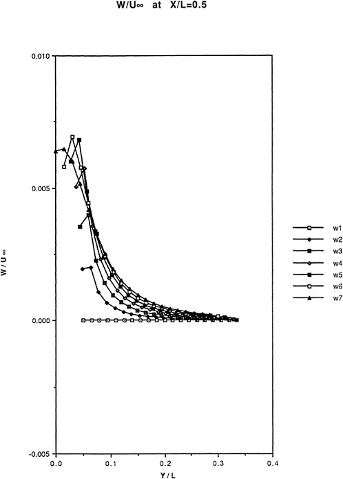
Velocity Field of a Source Distribution
The basic PDE given in (10) and (11) requires that U,V,W, and their first two derivatives with respect to y at y0, be calculated. Also, α(x,y0,z), and β(x,y0,z) defined in (4), and αx and βz at y0 must be computed. To obtain the latter quantities, the irrotational flow field within the region bounded by y0 and y2 is needed.
Hess, J.L. and Smith, A.M.O. [9] have furnished a formulation for calculating the velocity field for a flat quadrilateral panel on which a source distribution of constant strength is distributed. For forms such as Wigley's for which the potential can be expressed in terms of rectangular panels on the centerplane, it was possible to derive a much simpler set of formulas for U, V and W, by making one additional approximation. As in [4], we assume that the panels are flat; so that the direction cosines of the normals are constant on each panel, and that σQ'S on each panel are also constant. The additional approximation is that y0Q is replaced by y0-value corresponding to the center of the rectangle, y0c; i.e. a constant for each panel.
The velocity potential for a rectangular panel of dimensions 2a and 2b may now be written as

(21)
The results for U,V,W can be readily obtained by operating on the double indefinite integral, with ξ= xQ−xP, μ=y0Q−yP,ζ=zQ−zP,
(22)
Then
(23)
the constant of integration vanishing when the integration limits of (21) are introduced. Similarly
(24)
We also have
(25)
Then, introducing the integration limits in (23), we get
(26)
where
Similarly, from (25),

(27)
and from (24),

(28)
These expressions must be summed over all the panels for a fixed point P. Here we can again take advantage of symmetry in the y-z plane for 0<xc<L to collect four terms and to collect two terms for L<xc<2L with the same μc.
The approximation of replacing yQ in the integrations introduces appreciable errors in panels for points P close to a panel on y0. Since these constitute a small percentage of the total number of panels usually used, that error may be acceptable.
Velocity distributions computed from (26, 27, 28) are shown in Fig. 4.
SOLUTION OF STREAM-SURFACE EQUATION
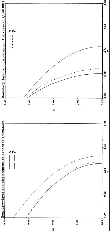
We can now consider a procedure for solving (10) and (11) for δ1. Initially, the case R=0, equivalent to Moore's PDE for thin boundary layers, was treated, i.e., with U∞=1,
Px+Qz=R
P=U0δ1−α Q=W0δ1−β (29)
with the boundary conditions
δ1(0,z)=0 at the bow
δ1z(x,0)=0 at the waterline by symmetry
δ1z(x,h)=0 at the keel by symmetry
Equation (29) was discretized by the method suggested by Lax [7]. The finite-difference formulation of (29) is

(30)
where
Here i and j denote indices for increasing values of x and z respectively. This gives a marching procedure in the x-direction. Using this formulation and the aforementioned boundary conditions, the case R=0 was solved. Typical results are shown in Figure 5. Since R was found to be very small, its effect on the calculated values of ![]() 1 was too small to show graphically. Thus, the thin-boundary-layer approximation is very good for the Wigley form.
1 was too small to show graphically. Thus, the thin-boundary-layer approximation is very good for the Wigley form.
ACKNOWLEDGMENT
The viscous-flow data for a Wigley form were furnished by Y.Tahara, computed for a turbulent boundary layer by a large-domain method. These data will be published among the papers generated by F.Stern 's viscous-flow program. For this and other assistance the authors are grateful to Tahara and Stern.
REFERENCES
1. Moore, F.K., “Displacement Effect of a Three-Dimensional Boundary Layer,” NACA Report 1124, 1953.
2. Lighthill, M.J., “On Displacement Thickness,” Journal of Fluid Mechanics, Vol. 4, Part 4, 1958, pp. 383–392.
3. Stern, F., Yoon, S.Y. and Patel, V.C., “Viscous-Inviscid Interaction with Higher-Order Viscous-Flow Equations, ” IIHR Report No. 304.
4. Hess, J.L. and Smith, A.M.O., “Calculation of Nonlifting Potential Flow About Arbitrary Three-Dimensional Bodies,” Douglas Aircraft Report E.S. 40622, 1962.
5. Kang, S.-H., “Viscous Effects on the Wave Resistance of a Thin Ship,” Ph.D. Thesis, The University of Iowa, July 1978.
6. Shahshahan, A. and Landweber, L., “Boundary-Layer Effects on the Wave Resistance of a Ship Model,” Journal of Ship Research Vol. 34, No. 1, March 1990, pp. 29–37.
7. Lax, P.P., “Weak Solutions of Nonlinear Hyperbolic Equations and Their Numerical Computations,” Communications on Pure and Applied Mathematics, Vol. 7, 1954.
8. Tikhonov, A.M. and Arsenin, V.Y., “Solutions of Ill-Posed Problems,” Published by V.H.Winston & Sons, Distributed by John Wiley & Sons, New York, 1977.
9. Landweber, L., “An Iteration Formula for Fredholm Integral Equations of the First Kind,” American Journal of Mathematics, Vol. 73, No. 3, July 1951.


DISCUSSION
by Professor F.Stern, University of Iowa, USA.
How well would your method of computing displacement bodies work with hull geometries that create more complex stern flows (i.e. Series 60 and HSVA tanker) than the Wigley hull?
Author's Reply
For application of our method to more ship-like forms, some of the special geometric properties of the Wigley form, of which we took advantage, would not be available. For example, the-turn-of-the-bilge is usually sharp for a merchant ship. When that is the case, the procedure of projecting the integral equation for the source distribution on the hull onto the vertical centerplane would have to be modified. That would complicate the discretization of the integral equation by means of flat panels. We would then prefer to use quadrature formulas instead of panels to compute the source distribution and its irrotational-flow field.
The more complex stern flows about ship-like forms would affect the determination of the viscous flow. Since we assumed that that flow was given, our method of determining the displacement thickness is unaffected. The same remark applies to bow flows (free-surface boundary layer, wave breaking, bilge vortices, necklace vortices).
Domain Decomposition in Free Surface Viscous Flows
E.Campana, A.Di Mascio, P.G.Esposito, and F.Lalli
(INSEAN, Italian Ship Model Basin, Italy)
ABSTRACT
In the present paper the computation of the steady free surface flow past a ship hull is performed by a domain decomposition approach. Viscous effects are taken into account in the neighbourhood of solid walls and in the wake by solving the Reynolds Averaged Navier-Stokes equations, whereas the assumption of irrotationality in the external flow allows a description by a potential model. Free surface boundary conditions have been implemented in a linearized form at the undisturbed waterplane. Suitable matching conditions are enforced at the interface between the viscous and the potential region. The numerical results obtained for the HSVA tanker and the S60 hull (Cb=0.6) are compared with experimental data, available in the literature.
NOMENCLATURE
|
B, B′ |
the wetted ship hull and its image |
|
D |
fluid domain |
|
Dp |
potential flow domain |
|
Dν |
viscous flow domain |
|
|
Froude number |
|
g |
acceleration of gravity |
|
H(x, y) |
free surface elevation |
|
J |
jacobian |
|
L |
ship hull length |
|
l |
unit vector tangent to the double model streamlines on z=0 |
|
l |
parameter defined along the double model streamlines on z=0 |
|
n |
unit vector normal to Г, oriented toward Dp) |
|
NNS |
number of iterations in the Navier-Stokes solver |
|
N=NS+NC |
number of boundary elements Lk used |
|
NS |
boundary elements arranged on S |
|
NC |
boundary elements arranged on Г |
|
P(x, y, z) |
field point |
|
p |
pressure |
|
p0 |
double model pressure |
|
Q≡(xQ, yQ, zQ) |
source point |
|
q≡(p, u, v, w) |
|
|
|
Reynolds number |
|
S |
free surface |
|
Sp |
free surface ∈ Dp |
|
Sν |
free surface ∈ Dν |
|
u=(u,ν,w) |
fluid velocity expressed in Cartesian components |
|
u0 |
double model fluid velocity |
|
U |
free stream velocity |
|
|
influence matrices |
|
Vn |
boundary condition for φ on Г |
|
|
boundary condition for |
|
x,y,z |
Cartesian coordinates in the body-fixed frame of reference |
|
β |
pseudo-compressibility coefficient |
|
Г |
interface between Dp and Dν |
|
Г* |
secondary interface (overlapping) |
|
εe |
fourth order artificial dissipation coefficient |
|
εi |
second order artificial dissipation coefficient |
|
ν |
kinematic viscosity of water |
|
νT |
eddy viscosity coefficient |
|
|
velocity potential (defined in Dp) |
|
φ |
potential of double model |
|
|
perturbation potential |
|
σ |
simple layer density for φ |
|
|
simple layer density for |
|
|
stress tensor |
INTRODUCTION
The prediction of the total drag of a hull in forward motion is a major task in ship design. To this aim, numerical fluid dynamics is a useful engineering tool for computing both pressure and viscous stresses on a body piercing the surface of the sea. Furthermore, it is possible to get detailed information on the wake past the hull; the knowledge of the velocity field in the aft region can help designers to improve the performance of the propeller and avoid cavitation.
However, the numerical simulation of this flow field is a difficult problem to deal with, because of the extremely large Reynolds numbers encountered in practical problems (∼ 108÷109), and the moving boundary at the air-water interface. The solution of the Navier-Stokes equations generally requires such a large amount of CPU time that this kind of codes becomes unfeasible for a customary usage in ship design. On the other hand, the codes based on potential flow models, although much faster than the former, are unable to mimic the formation and growth of the boundary layer and the wake.
In view of the problems mentioned above, the zonal approach concepts can be fruitfully exploited to save CPU time. In the proposed numerical algorithm the full viscous model is solved only in the neighbourhood of rigid boundaries and in the wake, while the external flow, where viscous effects are supposed to be negligible, is simulated by means of a potential model.
The present approach is quite different from the classical boundary layer-potential flow interactive methods based on the concept of displacement thickness. Applications of these schemes can be found in [1], where an integral boundary layer approach is used, or in [2], where the displacement thickness is computed by the solution of the Navier-Stokes equation close to the ship hull. In both cases, the boundary of the potential flow domain is determined by the displacement body. This kind of approach may cause some difficulties when dealing with full-form hulls and transom sterns, where the definition of the displacement thickness is not an easy task, especially when boundary layer separation occurs. In view of such applications, the present method is not based on the concept of displacement thickness, but we define a fixed decomposition of the fluid domain, with a matching surface located a priori. In ea ch domain, a suitable physical model able to grasp the relevant features of the flow is chosen and a proper numerical method is used: a Boundary Element Method is implemented for the solution of the external potential flow, whereas the Reynolds Averaged Navier-Stokes equations in the inner domain are discretized by a Finite Volume technique.
The Dawson model [3], in which the double model flow is the basis flow for the linearization, has been chosen for the free-surface external flow. The choice of a linear potential model is dictated by the need of CPU time saving; at the same time, the Dawson model was preferred with respect to other linear solvers because it allows a satisfactory representation of the free surface pattern also when dealing with full form hulls [4].
With a zonal approach, however, problems related to the matching conditions for the external and the internal solutions arise. Although the coupling procedure in unbounded flows is quite well established [5], the use of the zonal approach for solving free surface flows still needs to be investigated.
In the following sections, the viscous and inviscid solvers are described and the coupling procedure is analyzed. Finally some numerical examples are discussed and compared with experimental data.
MATHEMATICAL MODEL
In the following, we consider the steady flow around a rigid body B submerged or floating in an incompressible fluid of infinite depth, bounded upwards by a free surface S and unbounded in the other directions.
The fluid is assumed inviscid and the flow irrotational in the outer region Dp of the fluid domain D, whereas viscosity effects are taken into account in the inner region Dν (Fig. 1).

Figure 1: Computational sub-domains and overlapping zone
We assume a body-fixed reference frame with the x-axis oriented along the uniform stream U and the z-axis positive upwards.
The variables have been nondimensionalized with respect to the body length L and the uniform stream velocity U.
The Outer Region
The fluid velocity u=(u,ν,w) can be written as the gradient of a scalar function Φ:
u(x,y,z)=![]() Φ(x,y,z) (1)
Φ(x,y,z) (1)
The potential Φ, harmonic in Dp, is split into the double model term φ and the wave term ![]() :
:
(2)
The double model potential φ describes the flow past the body B and its image B′, symmetric with respect to the (x,y)-plane; namely, φz (x,y,0)≡ 0. The double model potential satisfies the Neumann BC's
![]() on Г (3)
on Г (3)
where Vn is the boundary condition to be specified later on, while Г is the matching surface.
At the free surface S : z=H(x,y) the pressure is constant, so that by Bernoulli's theorem we find the dynamic condition:
(4)
where surface tension has been neglected.
To get the linear form introduced by Dawson [3], we neglect the squares of ![]() ; if l is the curvilinear abscissa defined along the double model streamlines lying on z=0, the dynamic condition gives:
; if l is the curvilinear abscissa defined along the double model streamlines lying on z=0, the dynamic condition gives:
(5)
The linearized form of the kinematic condition, combined with (5), yields:
(6)
Therefore the wave potential can be computed by (6) on z=0 and by the following Neumann boundary condition:
![]() on Г (7)
on Г (7)
where ![]() is the boundary condition for the perturbation potential. Finally, the asymptotic behavior of the wave potential
is the boundary condition for the perturbation potential. Finally, the asymptotic behavior of the wave potential ![]() at infinity must be specified, i.e. waves should never propagate upstream. This gives the radiation condition:
at infinity must be specified, i.e. waves should never propagate upstream. This gives the radiation condition:
(8)
for every fixed (y,z) in Dp.
The solution of the mathematical model described above can be represented by means of a simple layer potential distributed over Г and the part Sp of the free surface included inside Dp [6]:
(9)
(10)
where P=(x,y,z) ∈ Dp, Q=(xQ,yQ,zQ) ∈ Г ∪ Sp, Q′=(xQ,yQ,−zQ).
Such definitions can be introduced in formulas (3) and (6–7), obtaining the integral equations whose discretization and numerical solution will be discussed in the next section. The double model potential can be computed independently by solving a standard Fredholm integral equation of the second kind for σ(Q).
The Inner Region
In the inner region Dν a turbulent viscous model has to be used to simulate the boundary layer growth and wake formation.
A pseudo-transient formulation due to Chorin [7] is used to solve the steady state incompressible Reynolds Averaged Navier-Stokes equations. In this scheme the continuity equation is replaced by a transient counterpart
(11)
where u=(u,ν,w) is the velocity vector expressed in Cartesian components, p is the pressure and β is the pseudo-compressibility factor. The resulting system of conservation laws is

(12)
where

(13)
In the previous equation ![]() is the stress tensor, including the turbulent part generated by the Reynolds averaging procedure. If an eddy viscosity turbulence model is introduced to evaluate the Reynolds stresses,
is the stress tensor, including the turbulent part generated by the Reynolds averaging procedure. If an eddy viscosity turbulence model is introduced to evaluate the Reynolds stresses, ![]() can be written as
can be written as
(14)
being Re the Reynolds number and νT the kinematic eddy viscosity. In the present paper the Baldwin-Lomax turbulence model [8] has been used.
If (ξ,η,ζ)=(ξ1,ξ2,ξ3) is a curvilinear coordinate system, equation (12) can be recast in the form
(15)
where J is the Jacobian and ![]()
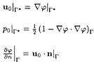
Apart the surface Г* at which the potential and the viscous solutions are matched, the boundary conditions imposed are the standard ones for Navier-Stokes computations. At solid walls no slip conditions are enforced, whereas at the mid-plane symmetry conditions are imposed:

(16)
At the outflow the velocity and the pressure fields are assumed to be fully developed, thus zero streamwise gradients are assumed. On the free surface, the boundary conditions to be satisfied are the following:

(17)
NUMERICAL MODEL
Potential Solver
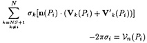
For the numerical solution of the problem described in the previous section, we discretize Г ∪ Sp into N=NS+NC plane quadrilateral elements Lk,k=1, …, N. NC denotes the number of panels located on Г and NS the number of those located on the average free surface Sp. Let P≡(x,y,z), Q≡(xQ,yQ,zQ) and Q′=(xQ,yQ,−zQ). The discrete form of the integral equation for σ(P) is the following:

(18)
for i=NS+1,…, N. Equation (18) can be rewritten in the following form:
(19)
where
(20)
(21)
The discrete forms of equations (6–7) are obtained:
(i=NS+1, …, N) (22)

(23)
where l(Pi) is the unit vector tangent to the direction l, and
In order to avoid numerical dispersion, we compute the derivatives of Vk(P) analitically; in fact the numerical dispersion can significantly affect the wave pattern, as shown in [6]. The radiation condition (8) is enforced in the following discrete form:
where j=1, …, Nj is the index set corresponding to all panels on the first upstream row. These equations replace the 2Nj equations (23) corresponding to the first upstream and the last downstream row.
Navier-Stokes Solver
A well established implicit scheme developed by [9] has been used in order to ensure reliable results and robustness needed for the interactive method.
A finite volume technique is used to discretize equation (12). The inner region Dν is divided in hexahedra Vijk. The application of the Gauss' theorem in the control volume Vijk yields
(24)
with
(25)
where Sijk is the boundary of Vijk, n= (nx,ny,nz) is the outer normal to Sijk and F= (F1,F2,F3). In the numerical approximation of equation (24) the values of F on the faces of cell Vijk are needed for the discretization of Equation (24): a simple averaging of neighbouring points is used to obtain velocity and pressure, while the stress tensor is evaluated by centered differencing.
The time marching procedure is that suggested by Beam and Warming [10]

(26)
where 0≤θ≤ 1. Using a Taylor expansion, equation (26) becomes

(27)
where δqn=qn+1−qn, Am and Bm,r are the jacobians of Fm:

(28)
A direct solution of the system of algebraic equations (27) would be too expensive, thus an approximate factorization technique is used to reduce it to the solution of three simpler problems, with block tridiagonal coefficient matrix:
(29)
within an accuracy of the order O(Δt). The operator A introduced in the factorization is defined as
(30)
with no summation on l. It can be noticed that all the second order mixed derivative in δq were discarded in the implicit part of the system to maintain the tridiagonal structure. This approximation, however, does not affect the steady state solution.
To improve the numerical stability of the scheme, a fourth order artificial dissipation term is added to the right hand side of (29). Thus the flux at the interface ![]() is modified according to
is modified according to
(31)
being ![]() is the average volume of the two neighbouring cells. A second order term is added to each tridiagonal operator in the left-hand side
is the average volume of the two neighbouring cells. A second order term is added to each tridiagonal operator in the left-hand side
(32)
(33)
The final form of the system of equations is, then
(34)
where ![]() is the residual that includes the artificial dissipation terms.
is the residual that includes the artificial dissipation terms.
It can be shown that the steady state solution is second order accurate and that the above scheme is unconditionally stable if θ≥0.5 in the linear case. The reader is referred to [9] and [10] for a detailed discussion.
In the implementation of the numerical code, all the metric terms in the above relations were computed in a finite volume fashion, i.e. the Jacobian Jijk was set equal to the volume cell Vijk and the terms like Jξi at the cell interfaces ξ=const., for instance, are computed as

(35)
where (nx,ny,nz) is the outer normal to the interface and ![]() is the area of the interface between (i,j,k) and (i+1,j,k).
is the area of the interface between (i,j,k) and (i+1,j,k).
A speedup in the computation can be achieved if a local time step is used
(36)
with C a stability parameter.
Applications of this scheme to ship flow calculation can be found, for instance, in [11] or in [12].
MATCHING ALGORITHM
The numerical algorithm used to couple the inner and the outer solution is the most important step of the whole procedure. The choice of the exchanged variables and the location of the matching surface may deeply affect the convergence rate or even cause the failure of the algorithm. In fact, in the previous version of the method [13], a non-overlapping domain decomposition scheme was used. The values of the tangential component of the velocity and the pressure of the potential field at the matching surface were used as boundary conditions for the Navier-Stokes solver, while the normal component of the viscous solution was used as Neumann condition in the potential flow. With this kind of approach, the convergence was reached within round-off errors but the convergence rate was not very satisfactory and some relaxation factors had to be used when matching the solutions. Furthermore, non-smooth transition from the inner to the outer domain was observed.
In the present work, the algorithm has been changed: the flow domain is divided in two subdomains that overlap over a small region, as illustrated in Fig. 1 for a two-dimensional case. These subdomains are bounded by Г and Г*, which are the boundaries in the flow field for the potential and viscous zones, respectively. The thickness of

Figure 2: Location of the exchanged variables at the matching interfaces
the overlapping region is equal to half the heigth of the outermost cells in the inner grid (Fig. 2). In the iterative coupling procedure, the solution computed in the first domain is used to feed the solution in the other domain with the boundary conditions, that is:
-
from the potential solver we get the velocity vector and the pressure at the grid point B on Г* (see Fig. 2); these values are forced as boundary conditions on the viscous flow

(37)
-
the normal component of the velocity at the control point A on Г (see Fig. 2) is computed from the viscous flow solution. This value is then used as a Neumann condition for the potential problem

(38)
This new scheme improves the convergence rate, makes the relaxation factors unnecessary and ensures a smooth transition across the matching surface.
However, the coupling procedure deserves a more detailed discussion. In fact, as mentioned before, the potential flow field is expressed as the sum of a double model potential φ and a wave potential ![]() . This linearized form [3], has been chosen because it gives a satisfactory description of the wave pattern also in case of non-slender hull, when compared with the Neumann-Kelvin linear problem. In order to keep the same representation of the potential flow, the multidomain solution has to be consistent with this decomposition, and therefore the solution is computed in two steps:
. This linearized form [3], has been chosen because it gives a satisfactory description of the wave pattern also in case of non-slender hull, when compared with the Neumann-Kelvin linear problem. In order to keep the same representation of the potential flow, the multidomain solution has to be consistent with this decomposition, and therefore the solution is computed in two steps:
-
Double Model Solution: The solution is computed with the condition
(39)
on the waterplane z=0, while the matching conditions on Г and Г* are
(40)
where u0 and p0 are the velocity vector and the pressure in the inner double model solution.
-
Free Surface Solution: Once the double model flow is solved with the desired accuracy, the free surface flow is computed. A linearised free surface condition is used in both domains on the water plane. However, the matching condition to be forced are slightly more complex than in the previous step. In fact, the potential
 is a perturbation with respect to the double model flow and therefore it must be related to the difference between the velocity field in the free surface viscous domain and the double model velocity field in the same domain. At the same time, the viscous solution, which is not split, must be related the total potential:
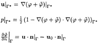
(41)
It is easy to verify that if (40) and (41) are summed, the global matching condition (37)–(38) are satisfied for the total potential Φ and the viscous solution (u,p).
The application of the multidomain decomposition technique in the form described above would be too much expensive. In fact, it implies the iterative solution of the Navier-Stokes equations for (u,p) assigned on Г* at each global step. This “inner” convergence seems not to be required when computing a steady state solution. In all the test cases we have performed, the Navier-Stokes solver was iterated for a fixed number N of steps (typically 1≤NNS≤100) and the algorithm never failed to converge. However, the number of sub-iterations affects the global convergence rate. We are not able to give a definite answer to this regard because only few test computations have been performed.
Finally, it is worth noticing that the CPU time spent in the computation of the potential solution is small compared to the total CPU time. In fact, the LU factorization of the matrix of the linear system for φ and ![]() is performed once, since the viscous solver only affects the RHS. Next inviscid steps are simply obtained by backsubstitution.
is performed once, since the viscous solver only affects the RHS. Next inviscid steps are simply obtained by backsubstitution.
NUMERICAL RESULTS
All the test cases presented in this section were computed with a workstation RISC/6000 Mod. 540 equipped with 128 Megabyte of RAM with peak performances equal to 60 MFLOPS.
Before the discussion of the numerical results, a few comments on the convergence behaviour of the algorithm may be worth doing. The procedure described above, as shown in Fig. 3, is consistent, in the sense that the discrete problem can be solved with any desired accuracy, up to round-off errors. The jump, clearly recognizable in the plot, is experienced when the free surface flow computation begin, starting from the converged double body flow. In this case (Wigley hull), 975 panels have been arranged on Г, 1050 panels on the undisturbed free surface, while the grid for the viscous problem is 65×15×15. However, in the applications such a fine resolution is not required: a tolerance equal to 10−3 generally suffices for practical purposes.

Figure 3: Convergence history of L2 norm of the mass residual
A Double Model Flow: the HSVA-tanker
The proposed algorithm has been applied in two different problems. At first, the coupling algorithm has been tested for a double model flow at Re=5×10⁶ past a typical bluff hull, such as the HSVA-tanker (Fig. 4); the grid in the viscous region is 65×14×14, while 910 panels are on the matching surface. In this test case Г is located at a distance from the hull equal to L/10, where L is

Figure 4: Computational grid showing part of the matching surface Г
the ship lenght. The potential solution is updated every NNS=10 viscous steps. The pressure contourlines on the hull have been depicted in Fig. 5:

Figure 5: Pressure contour map: comparison between present method (solid line) and full viscous solution (dashed line) for the HSVA-tanker. Levels: −0.5, −0.45, …, 0.5
the present method reproduces with a rather good agreement the results of the full viscous computation on a grid 80×30×24. The comparison of the performances of the two algorithm is very encouraging: the required CPU times are 4h with the zonal approach and 24h in the full viscous computation. In Fig. 6 the computed pressure is compared with experimental data ([14]). It can be seen that the agreement is quite good.

Figure 6: Pressure contour map: comparison between numerical results (top half) and and experimental data [14] (bottom half) for the HSVA-tanker. Levels: −0.5, − 0.475, ..., 0.5
A Free Surface Flow: the S60 Hull (Cb=0.6)

Figure 7: Computational grid showing part of the matching surface Г
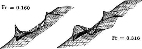
For the S60 Cb=0.6 model non-zero Froude number computations have been performed. Details of the grid can be observed in Fig. 7: the 77×25 free surface panels are arranged in a H-shaped grid that face the C-grid 70×15×15 in the viscous inner region. Numerical constraints related to both Reynolds and Froude number have to be satisfied in the grid spacing. In the computation reported in this sub-section, we have Re=4.5×10⁶ and Fr=0.300, 0.316. The grid lines were clustered at the hull surface to have a sufficient resolution in the boundary layer: the size of the first grid cell near the body is 10−5 in the normal direction. The nodes in streamwise direction were arranged to have at least 23 grid points per wave lenght (according to the linear 2D wave lenght formula). Regarding to the location of the matching surface, the viscous domain should be chosen as narrow as possible to improve

Figure 9: Top view of the boundary layer and the wake for the free surface flow
the efficiency of the numerical scheme in practical applications. In any case, all the relevant viscous effect must be confined inside the inner region. In the numerical tests, starting from a distance of L/2, Г has been moved closer to the body up to L/20. No significant changes in the solution have been observed. However, L/20 cannot be considered the closest distance at which Г can be located, since we have not performed further test cases. The analysis of this problem will be carried on more deeply in the future. In the computations reported in Figs. 8 and 9 (contour lines of the u components of the velocity for the double body flow and for Fr=0.316, respectively) it is shown that the boundary layer and the wake are clearly confined inside Dν.

Figure 10: Free surface elevation: comparison between numerical results (top half) and experimental data [16] (bottom half) for the S60−Fr=0.300. Levels of H/Fr2: −0.1, −0.09, …, 0.1
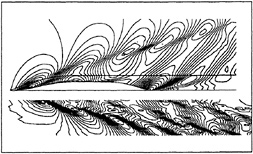
Figure 11: Free surface elevation: comparison between numerical results (top half) and experimental data [16] (bottom half) for the S60−Fr=0.316. Levels of H/Fr2: −0.1, −0.09, …, 0.1
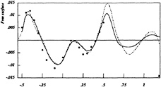
Figure 12: Free surface elevation along the hull at Fr= 0.300. — present method; - - - inviscid computation; •: experiment [16]
The wave patterns are shown in Figs. 10 and 11 for two values of Froude number: 0.300 and 0.316 (Re=4.5×10⁶). The computed solutions are compared with experimental measurements [15]. The inner and the outer solution seem to be very well matched, whereas the comparison with the experimental measured wave profiles is rather encouraging. Concerning the wave profiles along the hull, the potential solution (dotted line) seems to fit better the experimental data [15, 16] in the bow zone, with respect to the present solution (solid line). The rather unsatisfactory prediction at the bow may be due to the poor grid resolution, since only 15 points were used in girthwise direction. Upwind discretization of the free surface boundary condition in the inner region may be another cause of the bow wave underestimation.
Finally, the pressure on the hull surface at the stern is compared with measured values at Fr= 0.16 in Fig. 14. Also in this case, the numerical prediction is satisfactory.

Figure 13: Free surface elevation along the hull at Fr= 0.316. — present method; - - - inviscid computation; •: experiment [16]

Figure 14: Pressure at the stern of the S60 hull at Fr= 0.16: comparison between numerical results (solid line) and experimental data [16] (dashed line). Levels: −0.06, − .05, …, 0.1
CONCLUDING REMARKS
The numerical solution of a domain decomposition model for free surface steady viscous flows has been obtained; the preliminary results seem to be rather encouraging. The coupling algorithm between the viscous and the potential solvers is implemented by a robust iterative scheme. The CPU saving with respect to a full Navier-Stokes code is apparent and promising. Further numerical experiments are needed to analyze the dependence of the solution on the grid refinement and on the thickness of the viscous region. Moreover, in the viscous region, the wave amplitude is rather underestimated: this problem might be solved by a grid refinement, or by a more accurate implementation of the free surface boundary conditions for Navier-Stokes equations.
ACKNOWLEDGEMENTS
The work was supported by the Italian Ministry of Merchant Marine in the frame of INSEAN research plan 1988–90.
REFERENCES
[1] M.Ikehata, Y.Tahara, “Influence of Boundary Layer and Wake on Free Surface Flow around a Ship Model”, Nav. Arch. and Ocean Eng., Vol.26, p.71 ( 1988).
[2] Tahara, Y., Stern, F., “An Interactive Approach for Calculating Ship Boundary Layer and Wakes for Nonzero Froude Number”, Proc. XVIII O.N.R., Ann Arbor, Michigan, 1990.
[3] Dawson, C.W., “A Practical Computer Method for Solving Ship-Wave Problems”, 2nd Int. Conf. on Numerical Ship Hydro., Berkeley, 1977.
[4] Lalli, F., Campana, E., Bulgarelli, U., “Ship Waves Computations”, 7th Inter. Workshop on Water Waves and Floating Bodies, Val de Reuil, France, May 1992.
[5] Lock, R.C., Williams, B.R. ( 1987), “Viscous-Inviscid Interactions in External Aerodynamics”, Prog. Aerospace Sci., 24, pp.51– 171.
[6] Bassanini, P., Bulgarelli, U., Campana, E., Lalli, F., “The Wave Resistance Problem in a Boundary Integral Formulation”, to be published on Surv. Math. Ind..
[7] A.J.Chorin, J. Comput. Phys., Vol.2, pp.12– 26 ( 1967)
[8] Baldwin, B.S., Lomax, H. “Thin Layer Approximation and Algebraic Model for Separated Turbulent Flows”, AIAA Paper 78– 257, ( 1978)
[9] Kwak, D., Chang, J.L.C., Shanks, S.P., Chakravarthy, S.R., “A Three-Dimensional Incompressible Navier-Stokes Flow Solver Using Primitive Variables”, AIAA J., Vol.24, pp.390–396 ( 1986)
[10] R.M.Beam, R.F.Warming, “An Approximate Factorization Scheme for the Compressible Navier-Stokes Equations”, AIAA J., Vol.16, pp.393–402 ( 1978)
[11] Di Mascio, A., Esposito, P.G., “Numerical Simulation of Viscous Flows past Hull Forms”, The Second Osaka Inter. Coll. on Viscous Fluid Dyn. in Ship and Ocean Tech., Sept. 27–30, 1991
[12] Kodama, Y., “Grid Generation and Flow Computation for Practical Ship Hull Forms and Propelleres Using the Geometrical Method and the IAF Scheme” , Fifth International Conference on Numerical Ship Hydrodinamics, pp. 71–85, Hiroshima 1989
[13] Campana, E., Di Mascio, A., Esposito, P.G., Lalli, F., “Viscous-Inviscid Coupling in Ship Hydrodynamics”, XI Australasian Fluid Mech. Conf., Hobart (Australia), 1992.
[14] Knaack, T., Kux, J., Wieghart, K., “On the Structure of the Flow Field on Ship Hulls”, Osaka International Colloquium on Ship Viscous Flow, 1985
[15] Toda, Y., Stern, F., Tanaka, I., Patel, V.C. IIHR Report No. 326, Iowa Institute of Hydraulic Research, The University of Iowa, Nov. 1988
[16] Toda, Y., Stern, F., Longo, J., IIHR report No.352, Iowa Institute of Hydraulic Research, The University of Iowa 1991.
DISCUSSION
by Dr. Yoshiaki Kodama, Ship Research Institute, Tokyo, Japan.
I would like to congratulate the authors on this successful computation of free-surface flows using the domain decomposition method and ask the following questions:
-
On the free surface boundary of the inner region, five boundary conditions are needed, in agreement with the number of unknowns, i.e., u, v, w, p, and H (wave height). However, in Eq. (17) only four boundary conditions are given. What is the fifth boundary condition used?
-
Linearized free surface boundary conditions are used in the computations. How much does this approximation effect the computed results?
Author's Reply
We thank Dr. Kodama for his comments and discussions.
In response to the first question, on the free surface boundary of the inner region one of the unknown velocity components can be simply obtained by the continuity equation. The combination of this with the boundary conditions (17) give the complete set of conditions for the five unknowns.
Concerning the second question, it may be said that the limits of the linearized formulation re widely known, that is, its influence on the wave amplitude, wave shape and wave length. Aware of this, we decided to use the linearized formulation because of its simplicity. In fact, at the present stage of our research, we are mostly interested in the consequences of the use of the domain decomposition approach. We devoted our efforts in solving a few problems arising out of its use: the investigation on the effective CPU time reduction, on the smoothness of the solution at the matching boundary and on the robustness of the matching algorithm.
DISCUSSION
by Dr. P.M.Gresho, Lawrence Livermore National Laboratory, USA
In spite of your good-looking and converged solutions, I am disturbed by your matching boundary conditions for the viscous incompressible Navier-Stokes equations. You seem to specify all components of velocity and the pressure. The NS equations, however, are well-posed with just the velocity specified on the boundary of the solution domain (the pressure on the boundary is part of the solution!) and are over specified, and thus ill-posed, if you also specify the pressure. How do you account for this, or explain/justify you boundary conditions?
Author's Reply
Dr. Gresho is quite right, of course, regarding the number of boundary conditions to be imposed for the Navier-Stokes equations. At the matching boundary, continuity of pressure and normal velocity should be imposed, while a discontinuity on tangential velocity at the matching boundary should be allowed. However, in the overlapping region, we also expect the viscous term to be small and, moreover, the grid to be so coarse that viscous effects cannot be resolved. Therefore, for practical computation, we suppose that the model is the same on both domains in the overlapping zone, i.e., the algorithm works as if a homogeneous domain decomposition technique with overlapping were implemented.
The above discussion is not rigorous, being justified only on computational ground. From the theoretical point of view, doubts remain when the grid size goes to zero, in which case a discontinuity must be accepted on tangential velocity at the viscous-inviscid interface.
Interactive Zonal Approach for Ship Flows Including Viscous and Nonlinear Wave Effects
H.-C. Chen (Texas A&M University, USA)
W.-M.Lin and K.M.Weems
(Science Applications International Corporation, USA)
ABSTRACT
A hybrid numerical method for the prediction of ship flows including both viscous and nonlinear wave effects is presented. In this method, a zonal approach which combines a free-surface potential flow calculation and the Reynolds-Averaged Navier-Stokes (RANS) method is used. The linear potential flow calculation provides the ship-generated waves away from the ship. The RANS method in the near field resolves the turbulent boundary layer, the wake flows, and the nonlinear waves around the ship hull. The kinematic and dynamic free-surface boundary conditions are satisfied on the exact free surface in the RANS solution domain. The viscous-inviscid interaction is captured through a direct matching of the velocity and pressure fields in an overlapped RANS and potential flow computation region.
Extensive results are presented for the Series 60 CB=0.6 parent hull form at Froude numbers (Fr) =0.0 (double body), 0.160 and 0.316. The coupled RANS and potential flow method successfully resolves the hull boundary layer, the near wake, and the nonlinear free surface waves. The results clearly demonstrate the feasibility of the coupling approach and therefore enables us the use of a rather small RANS solution domain for efficient and accurate resolution of near-field ship flows.
INTRODUCTION
In the study of the body-wave interaction problems, potential flow methods are normally used. Viscous effects are included only empirically or in an integral sense to approximate overall viscous damping forces. This simplification in many cases is justifiable and also practically essential to keep the complexity of the problem in reasonable bounds. However, viscous effects are important to many ship free-surface flow related problems, such as roll motion, bow flow, stern flow and wake, detailed inflow to the propeller, and propeller/hull/wave interactions. In order to improve our understanding of the interaction between the viscous flow and wave field and to enhance our capability in the design and evaluation of new advanced ships, it is necessary to develop a prediction method which considers both the viscous and nonlinear wave effects.
In principle, both the viscous and wave effects can be calculated directly using the complete Reynolds-Averaged Navier-Stokes (RANS) equations for the entire flow field with an appropriate free surface boundary condition. This approach has been employed by Miyata et al. [1],[2] and Hino [3], among others, for ships in straight courses. These calculations, however, often require the use of a very large solution domain and an excessively large number of grid nodes to achieve adequate resolution of the entire flow field. Since the viscous effects are usually confined to a small region surrounding the ship hull and in the ship wake, it is desirable to use the simpler potential flow theories, instead of the complete RANS equations, for the wave field outside the viscous flow region. A zonal, interactive numerical approach which combines the RANS and potential flow calculations can therefore be an effective method for accurate resolution of ship free-surface flow problems.
The interaction among free-surface waves, the boundary layer, and wake flows has been the sub-
ject of many previous studies. Most of these studies, however, have focused on either viscous effects on wavemaking or wave effects on the boundary layer and wakes. A review of these works was given by, among others, Shahshahan & Landweber [4] and Stern [5]. More recently, Tahara et al. [6] and Toda et al. [7], [8] employed the displacement body concept of Lighthill [9] and developed an interactive approach to calculate ship boundary layers, wakes and wave field for a Wigley hull form. In their studies, the RANS method was coupled with the SPLASH free surface code of Rosen [10]. A simplified displacement body was used to account for the viscous effect in an approximate manner. The evaluation of displacement thickness, however, was found to be rather sensitive to small velocity changes in the outer part of viscous boundary layers. Furthermore, the validity of the displacement body concept also becomes questionable for problems involving thick boundary layers, wakes and/or regions of massive flow separation.
In view of the difficulties encountered in the displacement body approach, Chen and Lin [11] have explored several alternative coupling schemes including velocity/pressure matching, stream surface iteration, and field vorticity methods. Unlike the displacement body and the body vorticity methods proposed by Lighthill [9], these new coupling schemes do not rely on the thin boundary layer assumptions and are directly applicable to thick boundary layer as well as separated flow regions. Numerical results in Chen and Lin [11] for several axisymmetric bodies and three-dimensional double body ship forms clearly demonstrate that the velocity/pressure coupling scheme is the most accurate and efficient approach in capturing the viscous-inviscid interactions.
In this paper, the velocity/pressure coupling scheme is employed for the calculation of steady ship free-surface flow problems. The multiblock RANS method of Chen and Korpus [12] is extended for nonlinear free-surface flow calculations. Free surface potential flow methods are used to provide the wave field away from the ship hull. For the viscous-inviscid coupling, several major modifications are necessary for both the potential flow and the RANS methods. For completeness, the potential flow methods, the multiblock RANS methods, and the viscous-inviscid coupling scheme are briefly described. Calculations were performed using the Series 60 CB =0.6 parent hull form to examine the general performance of the interactive RANS and potential flow coupling method. Numerical solutions were obtained for the double-body flow (Fr= 0.0) and the steady ship free surface flow at Fr= 0.16 and 0.316. Detailed comparisons have been made with available experimental data to evaluate the general performance of the present interactive RANS/potential flow coupling approach.
POTENTIAL FLOW METHODS
For the solution of ship waves in the outer field, two potential-flow codes have been used. The SLAW (Ship Lift and Wave) code is a Dawson type steady ship wave panel code [13]. The LAMP (Large-Amplitude Motion Program) code utilizes a time-domain Green function approach [14]. Both methods and their respective advantages and disadvantages will be discussed here.
SLAW Calculations
The SLAW code was developed for computing the inviscid, irrotational, steady free surface flow around a ship operating on or near the free surface [13]. SLAW's basic formulation follows Dawson's method [15] for computing the hydrodynamic flow around a ship operating on the free surface. In this method, low order singularity panels are distributed over the body surface, SB, and a local region of the mean free surface, SF, as shown in Figure 1. Source panels are used for the free surface panels while body panels can either be source panels [16] for non-lifting problems or source and dipole panels [18] for lifting problems like sailing yachts running upwind. The lifting (source/dipole) singularity model includes dipole wake sheets for modeling vortex wakes and enforcing the Kutta condition on wake shedding edges.
SLAW satisfies an exact Neumann condition on SB and a linearized free surface boundary condition on SF, which is derived from the general form of the kinematic and dynamic free surface boundary conditions shown below:
(1)
(2)
where Φ is the velocity potential, n̂ the unit normal vector to the free surface, ζ(x,y) the
surface elevation, g the gravitational acceleration, and U∞ and V∞ are the x and y components of the inflow velocity at infinity. To linearize these conditions, Φ is divided into the double body potential, ΦDB, and a free surface perturbation potential, ![]() :
:
Φ=ΦDB+![]() (3)
(3)
After substituting this definition into Equations (1)–(2), higher order terms of the perturbation potential can be dropped to get the following linearized free surface boundary condition on the mean free surface:

(4)
In addition, a radiation condition must be imposed to avoid upstream waves. SLAW uses Jensen's upstream collocation point shift [17] technique to enforce the radiation condition, rather than upstream differencing used by Dawson and others. Since this technique eliminates the dispersion error and wave damping associated with the upstream differencing, SLAW's free surface solution is more suitable for the present zonal calculation than many other free surface potential flow methods.
Since the free surface boundary condition is linearized about the double body (Fr=0.0) flow, the double body potential is first calculated by imposing a normal velocity condition at the control point of each body panel:
(5)
where ![]() is the specified double body normal velocity and n̂ is the surface unit normal vector. The resulting system of linear equations can then be solved to get double body singularity strength for each body panel. Note that, because the double-body solution is solved separately and completely, SLAW is set up so that it can be used to compute Fr=0.0 problems (i.e. no free surface) simply by stopping the calculation after the double-body solution.
is the specified double body normal velocity and n̂ is the surface unit normal vector. The resulting system of linear equations can then be solved to get double body singularity strength for each body panel. Note that, because the double-body solution is solved separately and completely, SLAW is set up so that it can be used to compute Fr=0.0 problems (i.e. no free surface) simply by stopping the calculation after the double-body solution.
After the double body problem is solved, the perturbation potential is calculated by satisfying the linearized free surface boundary condition shown in Equation (4) at the control point of each free surface panel and the following perturbation velocity condition on each body panel:
(6)
where VN is the total specified normal velocity and ![]() is the double body specified normal velocity. The resulting system of linear equations can then be solved for the perturbation singularity strength on each body and free surface panel.
is the double body specified normal velocity. The resulting system of linear equations can then be solved for the perturbation singularity strength on each body and free surface panel.
Once the double body and perturbation singularities have been computed, flow quantities like potential, velocity, and pressure can be computed at field points anywhere in the fluid domain by calculating the influence of each panel on the specified field point. Note, however, that the edge singularity of the constant source and dipole panels make this type of influence calculation inaccurate for field points which are close (less then one half of a panel length) to a panel edge. For these cases, the field point quantities are interpolated from quantities computed at the panel control points and at field points “far” from panel edges.
SLAW Self-Consistency Test
For a conventional ship wave calculation, SB is simply the hull surface and the specified normal velocities, ![]() and VN, are zero for all panels. For the RANS/Potential Flow interaction problem where SLAW is being used to compute the outer flow region, SB is an arbitrary matching surface and the specified normal velocities,
and VN, are zero for all panels. For the RANS/Potential Flow interaction problem where SLAW is being used to compute the outer flow region, SB is an arbitrary matching surface and the specified normal velocities, ![]() and VN, are computed from the RANS solution for the inner flow region. Once either type of calculation has been done, the potential flow velocities and pressures on the RANS matching surface can be computed using SLAW's field point velocity routine. Special subroutines were added to the SLAW code to make the RANS/SLAW interaction virtually automatic.
and VN, are computed from the RANS solution for the inner flow region. Once either type of calculation has been done, the potential flow velocities and pressures on the RANS matching surface can be computed using SLAW's field point velocity routine. Special subroutines were added to the SLAW code to make the RANS/SLAW interaction virtually automatic.
Because the double body and total specified normal surface velocities, ![]() and VN, are specified separately, two procedures for matching the SLAW and RANS velocities are possible:
and VN, are specified separately, two procedures for matching the SLAW and RANS velocities are possible:
-
Compute an iterative RANS/SLAW double-body solution (Fr=0.0) first, using the double body RANS velocities on the matching surface as
 , then turn on the free surface effects, using the complete RANS velocity as VN.
-
Iterate between the complete (with free surface) RANS and SLAW solutions from the beginning, using the complete RANS velocity on the matching surface as
 and VN.
The first procedure has been used by Campana et al. [19]. The advantage of the this procedure is that it is completely consistent with the SLAW formulation. The disadvantage is that it requires iterating the RANS and SLAW calculations to convergence twice, first with the free surface effects neglected, and then with the free surface effects accounted for. The advantage of the second procedure is that its single iteration loop is simpler to implement and requires less computation. A possible disadvantage is that the specified normal velocities for SLAW's “double-body” solution, which are interpolated from the inner RANS solution, are no longer double-body (Fr =0.0) velocities. Numerically, this is no problem, since the free surface potential can be calculated as a perturbation about any basis potential solution. Likewise, the linearized free surface boundary condition used by SLAW will be valid for any basis potential as long as it has ![]() on z=0.0, which is implicitly satisfied by the singularity model used to compute the “double-body” flow. However, the RANS solution contains free surface effects and will not typically have
on z=0.0, which is implicitly satisfied by the singularity model used to compute the “double-body” flow. However, the RANS solution contains free surface effects and will not typically have ![]() at the mean free surface. In addition, the free surface effects in the RANS solution will appear in the nonlinear terms of the free surface boundary condition rather than the linear terms. Since it was not possible to predict a priori the effects of these “inconsistencies” on the SLAW calculation, a series of test calculations were done.
at the mean free surface. In addition, the free surface effects in the RANS solution will appear in the nonlinear terms of the free surface boundary condition rather than the linear terms. Since it was not possible to predict a priori the effects of these “inconsistencies” on the SLAW calculation, a series of test calculations were done.
In order to verify the validity of using the SLAW code to compute a zonal flow field and to investigate what velocity matching procedure was required, a series of test calculation were performed for a Wigley parabolic hull at Fr=0.340 in which the the SLAW code was used to calculate both the complete and the outer flow field. First, SLAW was used to compute the complete flow field, with the ship hull itself used as SB and the matching velocities, ![]() and VN, set to zero. The computed free surface elevation contours for this calculation are shown in the top plot of Figure 2. As part of this calculation, both double body
and VN, set to zero. The computed free surface elevation contours for this calculation are shown in the top plot of Figure 2. As part of this calculation, both double body ![]() and total
and total ![]() field point velocities were computed on a cylindrical “matching” surface which extended the entire length of the computational domain.
field point velocities were computed on a cylindrical “matching” surface which extended the entire length of the computational domain.
Two SLAW calculations were then made for the outer computation domain, with the “matching” surface used as SB. In the first outer domain calculation, the specified double body velocity on SB was set to be the normal component of the double body field point velocity computed in the complete domain calculation, and the specified total velocity SB was set to be the normal component of the total field point velocity:
(7)
(8)
This test calculation is the equivalent of the RANS/SLAW velocity matching procedure 1 above. Computed free surface elevation contours for this calculation are shown in the middle plot of Figure 2. These contours match the outer part of the complete domain contours almost exactly, confirming both the validity of the SLAW zonal calculation and the implementation of the field point velocity calculation and zonal interaction routines.
In the second outer domain calculation, both the specified double body and the specified total normal velocity on SB were set to the the normal component of the total field point velocity computed in the complete domain calculation:
(9)
This test calculation is the equivalent of the RANS/SLAW velocity matching procedure 2 above. The computed free surface elevations for this calculation are shown in the bottom plot of Figure 2. Again, these contours match the outer part of the complete domain contours almost exactly, verifying that SLAW zonal calculation can be made by matching the total velocity only and that first iterating to find the RANS/SLAW double body solution is not necessary. A similar zonal test calculation for the Series 60 hull confirmed that only the total velocity had to be matched.
LAMP Calculations
In our earlier study (Chen and Lin [20]), a three-dimensional time-domain program LAMP [14] was used. The LAMP code is generally used to compute the flow around a ship moving with forward speed in a seaway. In the LAMP approach, the exact body boundary condition is satisfied on the instantaneous wetted surface of the moving body while the free-surface boundary conditions
are linearized. The problem is solved using a panel method with distribution of the transient free-surface Green function for a step-function source below the free surface [21].
For the steady ship wave solution, the unsteady LAMP code is run for a ship started from rest and accelerated until it reaches a constant forward speed corresponding to the specified Froude number. The calculation is continued until a steady state is reached. It was found in [14] that the starting condition will affect only the initial transient behavior of the solution and has no effect on the steady-state solutions. For the RANS/LAMP interaction problem where LAMP is being used to compute the outer flow region, an arbitrary matching surface is used with the specified normal velocities computed from the RANS solution for the inner flow region.
The RANS/LAMP velocity-pressure coupling for the viscous free-surface flow problems was established by Chen & Lin in [20]. However, several issues remain to be addressed to ensure a general and robust RANS/LAMP coupling. First, the LAMP method, unlike the SLAW method described above, requires a closed matching surface which will have to cut through the viscous wake region. A discrete vortex model is needed in the LAMP computation domain to account for the viscous effect in the wake. Without the discrete vortex model, the LAMP solution can only be used for the initial “bare-body” calculation of velocities and pressures at the outer matching surface. Iteration between RANS and LAMP cannot be done. Secondly, the time-domain approach is computationally more expensive than SLAW for steady-state problems. However, the time-domain approach may be necessary for unsteady problems.
The numerical results obtained by RANS/LAMP coupling approach has been reported in details in Chen and Lin [20]. In the present study, we shall present only the potential flow results obtained by using the SLAW code.
MULTIBLOCK RANS METHOD
In the present study, the multiblock RANS method of Chen and Korpus [12] has been employed for the solution of viscous boundary layers, wakes and nonlinear free surface waves in the near field. We shall briefly describe the generalized RANS method in the following:
Governing Equations
Consider the nondimensional Reynolds-Averaged Navier-Stokes equations for incompressible flow in a orthogonal curvilinear coordinate system (x1,x2,x3,t):
(10)
(11)
where
and ![]() , and p represent contravariant velocities, Reynolds stresses, and pressure, respectively. The quantities gij and gij represent metric and conjugate metric tensors in orthogonal curvilinear coordinates, and the hi's represent associated metric scale factors. The Reynolds number Re=UoL/ν is based on a characteristic length L, a reference velocity Uo and the kinematic viscosity ν.
, and p represent contravariant velocities, Reynolds stresses, and pressure, respectively. The quantities gij and gij represent metric and conjugate metric tensors in orthogonal curvilinear coordinates, and the hi's represent associated metric scale factors. The Reynolds number Re=UoL/ν is based on a characteristic length L, a reference velocity Uo and the kinematic viscosity ν.
The Reynolds stresses are related to the corresponding mean rate of strain eij through an isotropic eddy viscosity νt,
(12)
(13)
where ![]() is the turbulent kinetic energy. The quantities eij and e(ij) represent contravariant and physical components of the rate-of-strain tensor respectively. Substitution into (11) yields momentum equations:
is the turbulent kinetic energy. The quantities eij and e(ij) represent contravariant and physical components of the rate-of-strain tensor respectively. Substitution into (11) yields momentum equations:

(14)
The quantity 1/Ru=1/Re+vt/σu represents the effective turbulent viscosity.
Equations (14) are closed using the two-layer turbulence model of Chen and Patel [22]. In the two-layer approach, the transport equations for
turbulent kinetic energy and its dissipation rate can be written as:
(15)
(16)
where
(17)
The effective viscosities in (15) and (16) are taken as 1/Rk=1/Re+νt/σk, and 1/Rε= 1/Re+νt/σε, respectively, and the coefficients (Cμ,Cε1,Cε2,σu,σk,σε) are fixed constants equal to (0.09, 1.44, 1.92, 1.0, 1.0, 1.3).
In the near-wall region, the rate of turbulent dissipation is specified in terms of k rather than being computed from (16). From Chen and Patel [22]:
(18)
where ℓε is a dissipation length scale equal to Cℓy[1−exp(−Ry/Aε)]. With k and ε known, the eddy viscosity is found from:
(19)
where
ℓμ=Cℓy[1−exp(−Ry/Aμ)]
The constants Cℓ, Aμ and Aε are chosen to yield a smooth distribution of eddy viscosity between the two regions, and take the values (Cℓ= ![]() , κ=0.418, Aμ=70, Aε=2Cℓ).
, κ=0.418, Aμ=70, Aε=2Cℓ).
For calculations around practical geometries, Equations (14) through (16) have been transformed into body-fitted coordinates t=![]() , xi= xi(ξ1,ξ2,ξ3,
, xi= xi(ξ1,ξ2,ξ3,![]() ):
):
(20)
(21)
(22)
(23)
where U(i)=hiUi are physical components of the contravariant velocity vector. The curvature parameters Kij, geometric coefficients αij, convection coefficients ![]() , source functions sφ and Laplacian operator
, source functions sφ and Laplacian operator ![]() 2, are given in Chen et al. [23].
2, are given in Chen et al. [23].
Multiblock Capability
In the present multiblock approach, the solution domain is first decomposed into a number of smaller sub-regions which are solved on a block by block basis. Within each computational block, the finite-analytic numerical method of Chen et al. [23] was employed to solve the unsteady RANS equations in a general curvilinear, body-fitted coordinate system. Complete continuity across block intersections is maintained by adding a one-cell overlap at each face. Thus, each point that is interior to the domain is also interior to at least one block. Block interface boundary conditions are updated by copying from the interior of adjacent blocks.
The current implementation requires continuity of grid lines across block faces, but not the one-to-one matching of the faces themselves. Any face can be divided into sub-sections that match different blocks, or that can be assigned different boundary conditions. Each block is allowed arbitrary dimension and orientation as long as the assembly of all blocks covers the entire solution domain. This multiblock structure has been further generalized in the present study to provide a flexible interface with the SLAW and LAMP codes in the potential flow computational block.
For three-dimensional flow calculations involving large number of grid nodes, a data management system was incorporated to circumvent the computer memory restrictions. The multiblock solution procedure requires only one block at a time, and reads the variables for that block as they are needed. Boundary data is stored in separate files since it may be needed a number of times during solution of any given block. The boundary files are relatively small, and can be read many times per iteration without slowing the computation. For the present interactive RANS/SLAW method, the SLAW solutions on any matching boundary can be readily treated as boundary data files in RANS calculations.
VISCOUS-INVISCID COUPLING
In the interactive RANS/SLAW calculations, the solutions in the RANS and SLAW solution domains are obtained separately. In order to capture the interaction between the viscous boundary layers and inviscid wave field, the velocity/pressure matching scheme developed by Chen and Lin [11] was employed to provide the viscousinviscid coupling between the RANS and SLAW solutions.
If the RANS solution domain is large enough to capture the entire viscous-inviscid interactions, it will not be necessary to update the SLAW solutions in the outer region. In practical applications, however, it is desirable to reduce the RANS domain to take full advantage of the efficiency and accuracy of the potential-flow solver, particularly for computing the inviscid wave field in free surface problems. When the RANS outer boundary is placed in the region where the interaction between the RANS and SLAW solutions remains significant, it is necessary to perform iteration between the RANS and the SLAW solutions so that the viscous effects on the free surface can be properly accounted for in subsequent SLAW calculations.
As noted earlier, the present velocity/pressure coupling scheme matches both the velocity and pressure fields directly at the matching boundaries. SLAW is run first to calculate the inviscid wave field for the bare hull. This provides the velocity and pressure boundary conditions for the RANS solver on the outer matching boundary embedded in the SLAW solution domain. The RANS method is then employed for the solution near the ship hull. The iteration between the RANS and the SLAW solutions is done by constructing an imaginary SLAW solution boundary (inner matching boundary) which lies outside the viscous boundary layers and wakes, but still embedded in the RANS solution domain. The SLAW solution is recomputed by using the matching surface as SB and the normal component of the RANS velocities as the specified SLAW normal velocities. Since the RANS normal velocities are used to specify the VN distribution for the SLAW calculations, the new far-field potential flow solutions will contain the influences of near-field viscous and nonlinear wave effects modeled in the RANS calculation.
In order to account for the viscous-inviscid interactions between the RANS and SLAW solutions, both the pressure and tangential velocity on the RANS outer boundary are matched directly to the SLAW solution. However, since the RANS and SLAW methods have different level of discretization errors, a direct matching of all three velocity components often leads to spurious pressure gradients along the RANS matching boundary. In order to ensure smooth pressure and velocity distributions between the viscous and inviscid flow domains, the normal velocity must be adjusted to eliminate any mass sources which may arise from incompatible pressure/velocity matching boundary conditions. In the present study, the SIMPLER/PISO coupling scheme has been modified to ensure the conservation of mass and momentum across block boundaries. In particular, the contravariant velocity components leaving (or entering) the matching face have been adjusted so that the continuity equation will be satisfied at all times. The modified SIMPLER/PISO scheme was then employed to compute the pressure field and update the velocity field in the RANS domain. The same procedure has also been used by Hubbard and Chen [24] in a Chimera RANS method to maintain smooth pressure and velocity distributions across arbitrary overlapping and embedding chimera grid blocks. A more detailed description of the modified SIMPLER/PISO pressure solver were given in Hubbard and Chen [24].
For double-body ship flows without the presence of free surface waves, the potential flow solutions can be obtained effectively even with large number of panels on the hull surface. This has been demonstrated in Chen and Lin [11] for SSPA 720 Cargo Liner using 1250 (50×25) hull panels and 1850 (74×25) off-body points on a cylindrical matching boundary locates at a distance of 0.1 ship length (L) from the centerline. In this case, the potential flow panelization corresponded exactly to the RANS surface grid. With the presence of the free surface effects, however, panels must also be distributed on the local pottion of the free surface, so it is necessary to reduce the number of hull and free surface panels in potential flow calculations in order to keep the computational efforts within reasonable bounds. In most calculations performed here, the SLAW panel distributions on the inner matching boundary were constructed by taking only the odd (2ξ1−1,2ξ3−1) nodes of the RANS numerical grid in the longitudinal and girthwise directions. The free surface panels were then automatically
generated by the SLAW code in order to resolve the ship wave. By generating the body panels in this manner, the specified normal velocities for the SLAW panels could be taken directly from the even (2ξ1,2ξ3) grid nodes of the RANS solution without resorting to interpolation.
Because of the needs for extensive refinement of hull and free surface panels at low speeds, the computational effort required for SLAW calculations increase rapidly at low Froude numbers. In addition, SLAW calculations have not been well validated at extremely low speeds. Detailed measurements by Toda et al. [7], [8], however, indicated that the free surface wave effects are negligible at low speeds except near the bow and stern. Since the viscous-in viscid interactions are quite weak at low Froude numbers, it is probably more effective to use a larger RANS solution domain and move the overlap region completely outside the interactive zone. This enables us to match the RANS solutions directly with bare-body SLAW solutions and avoid time-consuming RANS/SLAW interactive calculations. This non-interactive approach provides a powerful alternative to the SLAW or other potential flow codes for low speed simulations when the viscous effects are equally or more important than the wave effects.
Free Surface Boundary Conditions
As noted earlier, both SLAW and LAMP satisfy linearized free surface boundary conditions. In the initial phase of this study, the free surface boundary conditions in RANS domain were also linearized to simplify the coupling between the RANS and potential flow methods. Within the context of the linear wave theory, the dynamic and kinematic free surface boundary conditions were specified at the mean free surface of the RANS solution domain. Both the surface tension and viscous shear stresses on the free surface were neglected. The wave profile was calculated from the kinematic boundary conditions using a time-marching scheme. The pressure distribution on the mean free surface was then updated using the dynamic free surface conditions. Preliminary results exhibit some unrealistically large waves within the hull boundary layer. This is believed to be caused by the incompatibility of viscous boundary layer flow and inviscid wave field near the hull and free surface intersection. A detailed study of both the hull and free surface boundary layer including free surface turbulence is obviously needed in order to address the mixed-boundary shear flow in this region. Since such a study is well beyond the scope of the present research, we have adopt a rather crude approximation to treat this complex body/wave intersection problem. In the present study, this problem was circumvented by allowing the free surface within a small viscous layer (about 0.001 L) near the body to move like an inviscid flow with Neumann (zero gradient) boundary conditions.
In addition to the free surface and hull interaction problem, it was noted that the linearization of free surface boundary conditions also contributed to the under prediction of wave profiles at high Froude numbers. Measurements at Fr=0.316 by Toda et al. [7], [8] indicated that the maximum elevation change between the primary wave crest and wave trough amounts to nearly 50% of the ship draft. It is, therefore, desirable to apply the dynamic boundary condition on the exact free surface rather than the mean free surface for accurate resolution of viscous boundary layer and wake flows beneath the actual free surface. In the present study, the kinematic and dynamic free surface boundary conditions are applied on the exact free surface location. This is achieved by a simple stretching of the z coordinates in the vertical direction after a new free surface wave profile has been obtained from the integration of the exact kinematic free surface condition. It is recognized that this simple stretching procedure may lead to significant distortion of the hull forms. In order to minimize this distortion, the coordinate stretching was applied only to upper portion of the numerical grid near free surface while the remaining grids still conformed exactly with the original hull form. If more accurate representation of hull form is desired, it will be necessary to map the entire ship hull, including the exact hull geometry above the calm water level, into a parametric space. A parametric resplining of hull surface panels can then be performed to conform with the exact hull geometries. No such parametric resplining has been performed in the present study.
RESULTS AND DISCUSSIONS
In the present study, the RANS/SLAW method described above was employed for calculations of the viscous and wave fields around the Series 60 CB=0.6 parent hull. Calculations were performed for two different Froude numbers, Fr=
0.16 and 0.316, to facilitate a detailed comparison of numerical results with the velocity, pressure and wave elevation measurements documented in Toda et al. [7], [8]. For completeness, a double-body (Fr=0.0) calculation for the same hull has also been performed to quantify the effects of free surface waves at different Froude numbers. In this section, important numerical results are summarized and compared with available data for detailed assessment of the general performance of the present RANS/SLAW interactive approach.
Numerical Grid
In the present calculations for the Series 60 CB =0.6 parent hull form, a 85×36×29 body-fitted numerical grid shown in Figure 3 was employed to cover the entire viscous flow region. The grids was generated using an interactive gridding code GRIDGEN developed by Steinbrenner et al. [25]. The first station in axial direction was located at X/L=−0.5 upstream of the bow, and the last station was placed at X/L=2.0 in the wake where viscous diffusion is negligible. There are 49 streamwise and 29 girthwise stations on the hull itself. In addition, 12 stations were used upstream of the bow while 24 stations were employed for the resolution of ship wake flows. In the radial direction, 36 grid nodes were used between the hull surface and the RANS outer boundary located at R/L=0.3. The SLAW matching boundary was chosen to be constant-ξ2 coordinate surface with several grid-cells overlap between the RANS and SLAW solution domains. In double body calculations, the grid is uniformly distributed in the girthwise direction to provide appropriate resolution of the three-dimensional boundary layer on the ship hull. For non-zero Froude number cases, however, the numerical grids has been resplined to improve the resolution near free surface. In the present RANS calculations, the numerical grid was divided into four blocks to facilitate the implementation of the two-layer turbulence model and various boundary conditions. Furthermore, an extra station (ξ3=30) representing the mirror-image of ξ3=28 station was added on the other side of the keel plane (ξ3= 29) so that the flow on the keel plane can be calculated directly.
For nonzero Froude number calculations, it was necessary to adjust the solution domain to conform with the exact free surface profiles. As noted earlier, this was achieved by stretching only the upper portion of the coordinate surfaces beneath the free surface once the new wave profile is obtained from the integration of kinematic free surface boundary conditions. For high Froude number case considered here, the elevation change between the primary wave crest and trough can amount to about 50 % of the ship draft. Consequently, considerable grid adjustments are required in order to conform with the exact free surface profiles and resolve the nonlinear wave effects.
In the bare body SLAW calculations for double-body and Fr=0.316 cases, a 24×14 hull surface panel distribution was employed by selecting only the odd nodes from the RANS hull surface grid. The free surface panels were generated by adding 9 panels upstream and 17 downstream of the hull, and 21 panels in the transverse direction. This results in a total of 336 body panels and 882 free surface panels. For subsequent interactive calculations, the matching surface panels were again constructed by selecting the odd nodes from a constant-ξ2 coordinate surface in the RANS grid. The new free surface grid needed for SLAW calculations was generated by adding 2 stations upstream and 3 stations downstream of the matching surface panels. In the transverse direction, 19 panels were used with outer boundary located at Y/L=1.192. Overall, 588 (42×14) body panels and 855 free surface panels are used for the interactive SLAW calculations. Since the CPU time increases quadratically with the number of panels, the use of coarse panels enables us to reduce the run time to about 1/16 of the fine-grid calculations.
For the low Froude number (Fr=0.160) calculations, it was necessary to increase the number of body and free surface panels for proper resolution of the short wavelength, small amplitude free surface waves at low speeds. In the present bare-body SLAW calculations, the downstream boundary was placed at X/L=1.52 instead of 2.0 to reduce the computational efforts. On the hull surface, 840 (60×14) body panels were used to resolve the free surface waves. In addition, 2880 (96 ×30) free surface panels have been constructed by adding 8 panels upstream and 32 panels downstream of the hull. Since more panels and considerably longer run time will be needed for subsequent interactive calculations, it was decided to omit the interactive coupling between the RANS and SLAW solutions. As noted earlier, it is probably more effective to use a larger RANS solution
domain rather than performing RANS/SLAW interactive coupling for low speed calculations.
Interactive RANS/SLAW Coupling
Before describing detailed numerical results for the selected test cases, we shall carefully examine the general performance of the proposed velocity/pressure coupling approach with or without the presence of free surface waves. Interactive RANS/SLAW calculations were performed first for a double-body model of the Series 60 CB=0.6 parent hull at a Reynolds number Re=5×10⁶. Figure 4 shows the convergence history of the pressure along the waterline and wake centerline. It is seen that the solutions converged in just two interactive RANS/SLAW coupling cycles. Similar level of convergence has also been observed in our earlier RANS/LAMP calculations (Chen and Lin [11]) for other hull forms with much smaller RANS domain and stronger viscous-inviscid interactions.
The surface pressure distributions obtained by interactive RANS/SLAW method are in close agreement with the SLAW bare-hull solutions up to about 80% of the body length. The sharp reduction of hull pressure in the stern region is obviously due to the rapid thickening of hull boundary layers in that area. For completeness, the pressure and vertical velocity contours for both the non-interactive (zeroth iteration) and interactive (second iteration) solutions are shown in Figure 5 to further illustrate the effectiveness of the present interactive coupling scheme. The dashed (ξ2=30) and dotted (ξ3=36) lines in these plots represent, respectively, the inner SLAW and outer RANS matching boundaries. Only the outer part of the SLAW solutions were plotted in the overlap region since accurate evaluation of the off-body velocities in the vicinity of the body can only be achieved with local refinement of surface panels. In the non-interactive solutions, there are very significant differences between the RANS and SLAW solutions in the overlap region. The discrepancies are particularly noticeable in the stern region where the viscous effects has led to rapid thickening of the hull boundary layers. It is noted in Figure 5(c) that the RANS vertical velocities differ considerably from the corresponding potential flow solutions, indicating the presence of strong viscous effects. In order to properly account for the viscous effects, the RANS velocities normal to the matching boundary have been used to specify VN in subsequent SLAW calculations. This has led to dramatic improvement of the predicted vertical velocity contours near the SLAW inner matching boundary. Similarly, the modified SIMPLER/PISO scheme was also found to be very effective in maintaining smooth pressure distributions in the overlap region. The slight discrepancies in the overlap region are most likely due to the use of coarser matching surface panels in SLAW calculations.
It should be remarked here that, in double-body calculations, both the RANS and SLAW matching surfaces remain fixed. This enables us to match pressure and velocities directly on the same grid nodes without any interpolation. For nonzero Froude number calculations, however, the free surface grids in RANS solution domain have to be adjusted to provide accurate resolution of nonlinear free surface waves. On the other hand, the SLAW code still uses calm-water hull and free surface panels in the context of linear wave theory. This has caused some inconsistencies on both the SLAW and RANS matching boundaries since only the underwater portion of the hull geometry will be retained in SLAW calculations. In present implementation of velocity/pressure coupling approach, the two solutions have been matched in the transformed plane ξi without considering the actual grid deformations caused by nonlinear wave effects. This incompatibility can be readily removed if a fully nonliner potential flow method is used for the calculations of free surface waves in the far field.
Despite the inconsistencies mentioned above, the velocity/pressure coupling approach appears to be quite effective even for the high Froude number cases. This is clearly evident from the convergence history shown in Figure 6 for Fr=0.316 case. It is noted that the wave elevations along the waterline and wake centerline converged in just two to three RANS/SLAW iterations. The interactions between the viscous boundary layer and free surface flows completely altered the potential flow wave profiles in the stern and wake regions. In particular, the free surface waves decay very quickly along the wake centerline due to the convergence of low momentum fluid towards the ship stern and the centerplane of the wake. It is also seen from Figure 7 that the wave elevations along waterline and wake centerline (y=0) are rather insensitive to different choices of SLAW inner matching boundaries.
Figure 8 shows a detailed comparison of the axial velocity contours between the non-interactive and interactive solutions. The dashed and dotted lines again represent the SLAW and RANS matching boundaries. It should be remarked here again that the SLAW solutions were evaluated on the calm water surface z=0, while the RANS results were obtained on the exact free surface z=ζ. Since the amplitude of the primary wave amounts to about 25 % of the ship draft, the nonlinear wave effects and the associated grid deformations may lead to significant distortion of the plotted axial velocity contours. These must be borne in mind when comparing the linear SLAW and nonlinear RANS solutions in the overlap region.
The most notable feature of the non-interactive solutions shown in Figure 8 is the absence of the viscous wake in the bare-hull potential flow solutions. In addition, there is a rather abrupt change in the slope of non-interactive velocity contours near the RANS outer boundary. This is obviously caused by the stern boundary layer and viscous wake which occupied about 1/3 of the RANS solution domain. In particular, the viscous wake pushed the SLAW velocity contours away from the wake centerline and forced the formation of new axial velocity contours outside the viscous wake. Consequently, the interactive RANS/SLAW solutions shown in Figure 8(b) exhibit a weaker wave pattern with longer wavelengths in comparison with potential flow solutions. The interactive RANS and SLAW solutions are in fairly good agreement in the overlap region.
For completeness, detailed pressure and axial velocity contours are shown in Figure 9. For clarity, only the RANS solutions were plotted in the overlap region. Interactive RANS/SLAW calculations have been performed for two different inner matching surfaces at ξ2=30 (RANS/SLAW 1) and ξ2=32 (RANS/SLAW 2). It appears that the RANS/SLAW 1 matching surface may be too close to the viscous wake. The matching between RANS and SLAW solutions, however, improves significantly in RANS/SLAW 2 with the overlap region located outside the viscous wake. A systematic domain dependence study may be needed to guide the selection of both the inner and outer matching boundaries.
Finally, we shall examine some preliminary low Froude number (Fr=0.16) results to facilitate the discussion of Froude number effects. In potential flow calculations of low Froude number free surface flows, very fine panels and prolong simulation time are often required in order to resolve the short wavelength, small amplitude free surface waves observed at low speeds. Since the interaction between the far field free surface waves and the viscous boundary layers and wakes becomes quite weak at low Froude numbers, it is possible to neglect the free surface wave effects on the RANS outer boundary without significant effects on the viscous free surface flows in the near field. In our earlier RANS/LAMP calculations (Chen and Lin [20]), the near-field RANS solutions were matched directly with the double-body potential flow solutions to avoid lengthy time-domain LAMP computations. Although it appears that double-body matching conditions gave reasonable results for low Froude number simulations in the near field, it is still desirable to match the RANS solution directly with the potential flow free surface waves in order to ascertain the effects of matching conditions on the near-field viscous flow. A non-interactive RANS/SLAW calculation has been performed here to examine general features of the low Froude number free surface ship flows.
Figure 10 shows the numerical grid and calculated wave patterns for Fr=0.160 case. The SLAW free surface panels in the inner region was removed to facilitate the comparison of RANS and SLAW grid distributions. The potential flow wave patterns shown in Figure 10(b) reveals a quite complex system of short wavelength, small amplitude waves. It is evident that the RANS numerical grid must be refined in both longitudinal and transverse directions to provide adequate resolution of all detailed flow features at this Froude number. The refinement of RANS grid is currently in progress.
Despite the coarseness of the numerical grids, preliminary RANS calculations have been performed to examine the general features of near-field low Froude number flows. Figures 10(c) and 10(d) show the calculated axial velocity and pressure contours. The influence of pressure and velocity matching conditions on the RANS outer boundary appear to be confined to a narrow region and have very little effects on the near-field free surface flows. In view of this, we shall focus our attention on the near-field RANS solutions for the present study. It is also seen that the low Froude number results closely resemble the double-body
solutions except in the bow and stern regions. More detailed comparisons will be made in later sections for further assessment of the near field solutions.
Double-Body Results
In order to facilitate a direct comparison of free surface wave effects between low and high Froude numbers cases, we shall present both the Fr= 0.160 and 0.316 results in the same plots. Furthermore, comparisons will also be made with double body solutions for more detailed examinations of complex interactions between the turbulent boundary layers, ship wakes and nonlinear free surface waves. For simplicity, we shall examine first the double-body turbulent boundary layer and wake flows without the complications due to surface waves. This enables us to establish a baseline solution for the assessment of free surface wave effects. In this section, we shall discuss only the basic flow features associated with double-body models. All the double-body solutions are shown as part (a) in Figures 11 through 14 to facilitate the comparisons and discussion of free surface effects at different Froude numbers.
Figure 11(a) shows the calculated double body pressure and axial velocity contours on the hull surface as well as the waterline and keel planes of symmetry. The pressure and axial velocity contours at selected transverse sections are shown in Figures 12(a) and 13(a). Together, they provide a detailed description of the three-dimensional pressure and axial velocity fields. For the double-body models considered here, strong pressure variations were observed in both the bow and stern regions due to the rapid changes of hull geometry in these areas. In the absence of free surface waves, it is seen that the boundary layer remains thin up to about 80% of the ship hull. Beyond that, a thick boundary layer develops quickly due to rapid changes in stern geometry and the accompanied three-dimensional pressure gradients around the hull surface.
Figure 14(a) shows the transverse velocity vector plots at several axial stations. The complex secondary flow patterns were generated by the geometrically-induced pressure gradients in the girthwise direction. The present solutions successfully captured the development of the bow bilge vortex (x=0.4), the convergence of crossflow in the stern region (x=0.8 & 0.9), and the evolution of the stern bilge vortex in the near wake (x=1.1). The convergence of the crossflow in the stern region is responsible for the thickening of stern boundary layer and near wake flows shown in Figure 13(a).
Nonzero Froude Number Results
Measurements performed recently by Toda et al. [7], [8] for the Series 60, CB =0.6 parent hull indicated very significant differences between the high and low Froude number data due to the wave-induced effects. In general, both the amplitude and length of the ship generated waves increase as Froude number becomes higher. At Fr=0.16, the free surface effects are negligible except near the bow and stern regions. The measured pressure and velocity profiles also resemble those for the double body ship models. At higher Froude number of 0.316, the interactions between the viscous boundary layer, wake and free surface waves become much more profound near the bow, the afterbody, and in the wake. In these areas, both the viscous and free surface flows are significantly altered due to boundary layer, wake and wave interactions.
As described earlier, calculations have been performed for both Fr=0.160 and 0.316 cases to examine the free surface effects. For the Fr= 0.160 case, we shall focus only on the comparison of near field flows. Figure 11 shows a comparison of pressure and axial velocity contours at different Froude numbers. At the low Froude numbers, it is seen that the pressure on the free surface differs considerably from that for the double-body case. But the wave effects was clearly confined to a small layer just beneath the free surface. This is also evident from Figure 12(b) which shows the pressure contours on several transverse sections. Note that the pressure contours on each transverse section are nearly identical to the corresponding double-body results shown in Figure 12(a) except in a small region just below the free surface. The wave-induced pressure gradients, however, are very large within this small surface layer.
Figure 13(b) and 14(b) show the axial velocity and crossflow vectors at several transverse stations. As expected, the influence of the free surface waves was also seen to be confined to a thin surface layer. It is interesting to note that the vertical velocity component changes rather dras-
tically near the free surface even though the crossflow patterns returned quickly to the double-body pattern underneath the free surface. The magnitude of the surface vertical velocity is, in fact, comparable to that obtained for Fr=0.316 case and is directly associated with the large wave-induced pressure gradients near the free surface. Both the crossflow patterns and the wave-induced pressure gradients can be explicated by the wave elevations shown in Figure 15.
With the increase of Froude number or ship speed, both the free surface wave elevations and wavelengths increase. As can be seen clearly in Figures 12 through 14, the wave elevation has large difference at x=0.1 and at x=0.4. Note that the amplitude of the bow wave is about 25 % of the ship draft. It is also seen from perspective views shown in Figures 15 and 16 that the nonlinear free surface waves induced very strong pressure gradients, both in the longitudinal and transverse directions. The presence of these wave-induced pressure gradients have led to significant modifications of the viscous boundary layer and wake flows shown in Figures 13 and 14. Compared to the Fr=0.160 results, the wave-induced effects were also observed to penetrate much deeper into the fluid domain. Both the pressure and velocity contours plots reveal a strong interaction between the viscous boundary layer and wake, and the nonlinear free surface wave field. Most of the interaction can again be explicated as a result of the wave elevations and the wave-induced pressure gradients. For completeness, the free surface profiles are shown in Figures 15 and 16 to facilitate the discussion of wave-induced effects.
For high Froude number case, the wave-elevation contours reveal complex wave patterns consisting of both transverse and diverging wave systems. Close to the hull surface, it is seen that both the bow- and stern-wave systems were initiated with crests and the shoulder wave systems with troughs. Away from the ship hull, there is a complex interaction between the bow-, shoulder-and stern-wave systems, which creates the overall wave patterns shown in Figures 15 and 16. Compare to the Fr=0.160 results, there is a much more distinct diverging wave system, especially in the bow and stern areas. Furthermore, it is also evident from the pressure contours shown in Figures 11 and 12 that the wave-induced pressure gradients remained very significant for a large portion of the underwater hull surface. These pressure gradients are responsible for the development and evolution of crossflow patterns shown in Figure 14. It is quite clear that the wave-induced effects have altered both the magnitude and direction of the crossflow vectors up to about 50% of the ship draft.
Figure 15 shows the nonlinear waves in the RANS solution domain. A perspective view of the complete wave patterns in both the RANS and SLAW domains are also shown in Figure 16. The wave elevations were normalized by 1/Fr2 to reveal the complex wave patterns for both cases. The actual wave elevation for Fr=0.160 case is about 1/4 of that for the high Froude number Fr= 0.316 case. At Fr=0.160, the hull surface pressure is nearly identical to those calculated for the double-body model. The wave effects on the viscous boundary layer and wake flows are rather small, except in the bow and stern areas. The wave pattern itself, however, is quite complex in the near field. For double body calculations, the wave field will be completely suppressed by requiring the vertical velocity to be zero on the free surface. This can only be achieved with a nonzero pressure field (i.e., the double-body pressure) on the mean free surface. For nonzero Froude number calculations, on the other hand, the dynamic free surface boundary condition requires the total pressure to be zero (i.e., equal to ambient pressure) on the free surface. In practice, no matter how small the Froude numbers are, gravity waves must be generated in order to balance the fictitious double-body pressure gradients on the free surface. Note that the dynamic pressure on the free surface is always proportional to the wave elevation, normalized by Fr2, when both the surface tension and viscous stresses are neglected. At low Froude numbers, the dynamic pressure returns rapidly from the free surface values to the double body distributions within a small surface layer. Therefore, a large wave-induced pressure gradient is produced across the surface layer. This leads to the development of large vertical velocities observed in Figure 14 near the free surface.
Finally, the calculated and measured wave profiles along the ship hull are shown in Figure 17 for both Froude numbers. For Fr=0.160 case, the wave elevations predicted by the non-interactive RANS method are in excellent agreement with the measured data in the bow and forebody regions. The wave elevations for the afterbody, however, was somewhat underpredicted. The underprediction in the stern region is most likely
caused by the inadequate grid resolutions noted earlier. For completeness, the bare-hull potential flow wave elevations are also shown in Figure 17(a) to quantity the viscous effects. It is seen that the viscosity plays a dominant role in eliminating the short wavelength, small amplitude waves at low speeds.
For high Froude number (Fr=0.316) case, it is seen from Figure 17(b) that the wave elevations obtained by interactive RANS/SLAW method are in very good agreement with the measured values over the entire ship. The bare-body potential flow solutions overpredicted the wave elevation in the stern region, but underpredicted the amplitude of the primary wave in the bow region. The overprediction of stern waves is obviously due to the negligence of viscous effects due to thick boundary layer and wake flows. The underprediction of the bow wave, however, must be attributed to the use of linearized free surface conditions in SLAW bare-body calculations. It is noted that the wave elevation changes by as much as 0.03 of ship length or 50% of the ship draft. Although this wave amplitude may still be considered small compared to wavelength, it is quite clear that the viscous boundary layer and wake flows will be greatly influenced by the nonlinearity in the free surface wave field. Consequently, it is necessary to adjust the RANS solution domain in order to properly account for the nonlinear wave effects due to local changes in underwater geometry at each transverse section.
It should be emphasized that both the viscous and wave effects have been included directly in the present RANS calculations, even though the surface tension and viscous stresses on the free surface had been neglected due to a lack of understanding on the physical processes and mathematical modeling of the free surface turbulence. The inclusion of both the viscous and wave effects enables us to capture the complete interaction between the wavemaking and viscous boundary layer and wake in the near field. In particular, the wave-induced effects were formally included by requiring the dynamic free surface boundary conditions to be satisfied on the exact free surface. On the other hand, the influence of viscous boundary layer and wake flows on the free surface waves was captured automatically when the kinematic boundary conditions were used to update the free surface wave profiles.
CONCLUSIONS
An interactive numerical method which combines the Reynolds-Averaged Navier-Stokes (RANS) method and the free-surface potential flow calculations has been developed for the prediction of ship flows including both the viscous and nonlinear free-surface wave effects. In this zonal approach, the RANS method is employed to resolve the viscous boundary layer, wake and the nonlinear free-surface waves around the ship hull while the potential flow method is used to provide the wave information outside the viscous region. For high Froude number cases where the wave effects are significant, the near-field RANS solution is matched with the SLAW solution. Iterations between the two solutions are performed to capture the interaction between the viscous and the wave effects. Only one to two iterations is needed to achieve a converged solution. At low Froude numbers, the wave effects outside the RANS domain are insignificant and the RANS solutions are matched with the SLAW solution without iteration.
In the present RANS calculations, the dynamic free surface boundary conditions are satisfied on the exact free surface and, therefore, it is possible to capture the strong interaction between the nonlinear waves, the boundary layer, and wake flows underneath the exact free surface. With further modifications in the adaptive grid generation procedure, the present method can be readily generalized for the prediction of nonlinear wave effects arose from arbitrary ship motions.
Calculations have been performed for the Series 60, CB=0.6 parent hull for both low and high Froude number causes. The numerical solutions clearly demonstrated the feasibility of coupling the RANS and SLAW methods in an interactive approach for detailed resolution of both the viscous and the free-surface wave effects. This enables us to use a rather small RANS solution domain for efficient and accurate resolution of the interaction between wavemaking and viscous boundary layer and wake.
All of the RANS calculations presented here were performed on CRAY YMP supercomputers. The CPU time required is about 440 CPU seconds for every 100 time steps. Normally, 200 to 300 times steps are needed to achieve complete convergence for a non-interactive solution. In the subsequent interactive calculations, 50 to 100 more time steps
were used for each interactive RANS/SLAW coupling solution. A complete RANS calculation for the near-field viscous flow with three interactive coupling cycles takes about 30 to 45 CPU minutes. The SLAW calculations for double-body and Fr=0.316 cases were performed on an IRIS R4000 –50 GTX workstation, while the Fr= 0.160 results were obtained on a IBM RS6000/550 workstation. Depending on the Froude Number, the SLAW calculations of the potential flow waves take about 5 to 80 (Fr=0.160 case) CPU minutes for one solution on the workstations. In general, a complete RANS and potential flow coupling solution may be obtained in less than 1 CPU hour on a CRAY YMP. This demonstrates the efficiency of the method presented in this paper and shows the feasibility of using this type of advanced numerical method for evaluation of practical problems.
The method developed in the present study is very general. With the present velocity/pressure coupling approach, it is possible to use the most suitable and efficient solver for each different flow region to provide maximum flexibility, accuracy and efficiency. With some modifications, the method can be readily generalized for the study of nonlinear unsteady interaction of ship and waves, effect of propulsor on stern flows, and other near-field ship flow problems.
ACKNOWLEDGEMENT
This work has been supported by the Office of Naval Research under the Nonlinear Ship Motion Program Grant N00014–90–C–0031, monitored by Mr. James A.Fein. Some of the results reported in this paper have been obtained under the support of the Advanced Research Project Agency (ARPA) Submarine Technology Program monitored by Mr. Gary Jones. Most of the computations were performed on the CRAY Y-MP8e/8128 –4 of Cray Research Inc. at Eagen, Minnesota under the sponsorship of Mr. Chris Hempel. Preliminary developments of the computer codes were done on the CRAY Y-MP2/116 at the Texas A & M Supercomputer Center through a Cray Grant provided by Cray Research Inc.. We are grateful to Cray Research Inc. for the use of these computing resources.
References
[1] Miyata, H. and Nishimura, S., “Finite-Difference Simulation of Nonlinear Waves Generated by Ships of Arbitrary Three-Dimensional Configuration,” Journal of Computational Physics, Vol. 60, No. 3, pp. 391–436, 1985.
[2] Miyata, H., Zhu, M. and Watanabe, O., “Numerical Study on a Viscous Flow with Free-Surface Waves About a Ship in Steady Straight Course by a Finite-Volume Method,” Journal of Ship Research, Vol. 36, No. 4, pp. 332–345, 1992.
[3] Hino, T., “Computation of a Free Surface Flow around an Advancing Ship by the Navier-Stokes Equations,” Proc. 5th International Conference on Numerical Ship Hydrodynamics, 1989, Hiroshima, Japan.
[4] Shahshahan, A. and Landweber, L., “Interactions Between Wavemaking and the Boundary Layer and Wake of a Ship Model,” IIHR Report No. 302, 1986, Iowa Institute of Hydraulic Research, The University of Iowa, Iowa City, IA.
[5] Stern, F., “Effects of Waves on the Boundary Layer of a Surface-Piercing Body, ” Journal of Ship Research, Vol. 30, No. 4, pp. 256–274, 1986.
[6] Tahara, Y., Stern, F. and Rosen, B., “An Interactive Approach for Calculating Ship Boundary Layers and Wakes for Nonzero Froude Number,” Proc. 18th ONR Symposium on Naval Ship Hydrodynamics, 20–24 August, 1990, Ann Arbor, MI.
[7] Toda, Y., Stern, F. and Longo, J., “Mean-Flow Measurements in the Boundary Layer and Wake and Wave Field of a Series 60 CB =.6 Ship Model for Froude Numbers .16 and .316,” IIHR Report 352, 1991, Iowa Institute of Hydraulic Research, The University of Iowa, Iowa City, Iowa.
[8] Toda, Y., Stern, F. and Longo, J., “Mean-Flow Measurements in the Boundary Layer and Wake and Wave Field of a Series 60 CB =.6 Ship Model—Part 1 : Froude Numbers .16 and .316,” Journal of Ship Research, Vol. 36, No. 4, pp. 360–377, 1993.
[9] Lighthill, M.J., “On Displacement Thickness,” J. of Fluid Mechanics, Vol. 4, Part .4, 383–392, 1958.
[10] Rosen, B., “SPLASH Free Surface Code : Theoretical/Numerical Formulation,” South Bay Simulation Inc., Babylon, NY, 1989.
[11] Chen, H.C. and Lin, W.M., “Interactive RANS/LAMP Coupling Schemes and Their Applications to Ship Flows,” SAIC-91/1021, February 1991, Science Applications International Corporation, Annapolis, MD.
[12] Chen, H.C. and Korpus, R., “A Multi-block Finite-Analytic Reynolds Averaged Navier-Stokes Method for 3D Incompressible Flows,” Proc. ASME Fluid Engineering Conference, Washington, D.C., June 20–24, 1993.
[13] Letcher, J., Weems, K., Oliver, C., Shook, D., and Salvesen, N., “SLAW: Ship Lift and Wave, Theory, Implementation, and Numerical Results , SAIC Technical Report 89/1196, 1989.
[14] Lin, W.M. and Yue, D.K.P., “Numerical Solutions for Large-Amplitude Ship Motions in the Time-Domain ”, Proc. 18th Symp. Naval Hydro., The University of Michigan, Ann Arbor, MI, USA, 1990.
[15] Dawson, C., “A Practical Computer Method for Solving Ship-Wave Problems” Proc, 2nd International Conference on Numerical Ship Hydrodynamics, University Extension Publishers, Berkeley, CA, 1977, pp 30–38.
[16] Hess, J., and Smith, A., “Calculation of Nonlifting Potential Flow about Arbitrary Three-Dimensional Bodies”, Journal of Ship Research, Vol 8, 1964, pp 20–24.
[17] Jensen, P., “On the Numerical Radiation Condition in the Steady-State Ship Wave Problem”, Journal of Ship Research, Vol 31, pp 14–22, 1987.
[18] Morino, L., Chen, L.-T., and Suciu, E., “ Steady and Unsteady Oscillatory Subsonic and Supersonic Aerodynamics around Complex Configurations” , AIAA Journal, Vol 13, pp 368–374, 1975.
[19] Campana, E., Di Mascio, A., Esposito, P.G., and Lalli, F., “A Multidomain Approach to Free Surface Viscous Flows”, Abstract submitted to the Eighth International Workshop on Water Waves and Floating Bodies, St. John's, Newfoundland, Canada, May 1993.
[20] Chen, H.C. and Lin, W.M., “Interactive RANS/LAMP of Ship Flows Including Viscous ans Wake Effects, ” SAIC Technical Report 92/1049, 1992.
[21] Stoker, J.J., “Water Waves,” Pure and App. Math., Volume IV., 1957.
[22] Chen, H.C. and Patel, V.C., “Near-Wall Turbulence Models for Complex Flows Including Separation, ” AIAA Journal, Vol. 26, No. 6, pp. 641–648, June 1988.
[23] Chen, H.C., Patel, V.C. and Ju, S., “Solutions of Reynolds-Averaged Navier-Stokes Equations for Three-Dimensional Incompressible Flows,” Journal of Computational Physics, Vol. 88, No. 2, pp. 305–336, 1990.
[24] Hubbard, B, and Chen, H.C., “A Chimera Reynolds-Averaged Navier-Stokers Methods for 3D Incompressible Flows,” Texas A & M Research Foundation, COE Report No. 328, 1993.
[25] Steinbrenner, J.P., Chawner, J.R. and Fouts, C.L., “The GRIDGEN 3D Multiple Block Grid Generation System,” Vols. I & II, WRDC-TR -90–3022, 1990, Wright Patterson AFB, OH.
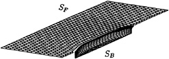


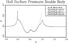


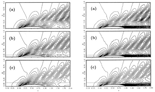
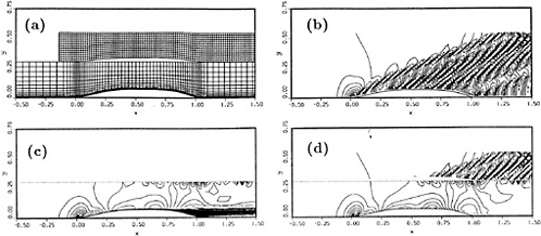
Fig. 10: Fr=0.160 Solutions: (a) Numerical Grid, (b) Bare-Hull SLAW Wave Patterns, (c) RANS Axial Velocity Contours, (d) RANS/SLAW Pressure Contours.

Fig. 11: Pressure (left) and Velocity (right) Contours: (a) Interactive Double-Body, (b) Non-interactive Fr =0.160, (c) Non-interactive Fr=0.316, (d) Interactive Fr=0.316.